February 2008
In this Issue:
Two control charts used with yes/no type data are the p and np control charts. We usually collect the data and then calculate the average and the control limits, either manually or with software. But did you know that the control limit equations for the p and np control charts are only valid under certain conditions? The equations are not valid when you have what is called the “small sample case” for p and np control charts. This newsletter discusses this small sample case and how the control limits are determined.
p and np Control Charts
p and np control charts are used with yes/no type attributes data. These two charts are commonly used to monitor the fraction (p chart) or number (np chart) of defective items in a subgroup of items.
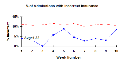
With this type of data, there are only two possible outcomes: either the item is defective or it is not defective. For example, suppose you are using a p control chart to track the fraction (or %) of hospital admissions that had incorrect insurance information each week. There are only two possible outcomes: either the admission had the correct insurance information or it did not have the correct insurance information. This type of data is referred to as yes/no data. It either meets some preset specification (yes) or it does not meet the preset specification (no). You would collect data each week on the number of hospital admissions (n, the subgroup size) and the number with incorrect insurance information (np, the number defective). Each week you calculate the fraction defective, p, which is equal to np/n. The values of p are plotted over time. Once enough data is available, you calculate the average (pbar) and control limits (LCLp and UCLp). For more information on p control charts, please see our July 2005 newsletter that is available on our website.
If the subgroup size is the same each time, the np control chart can be used in place of the p control chart. In this case, the number of defective items (np) is plotted over time. Again, once enough data is available, you calculate the average (npbar) and control limits (UCLnp and LCLnp).
- Both these charts involve counts. You are counting items. To use a p or np control chart, the counts must also satisfy the following two conditions:
- You are counting n distinct items. np is the number of items in those n items that fail to conform to specification.
Suppose p’ is the probability that an item will fail to conform to the specification. The value of p’ must be the same for each of the n items in a single sample.
If these two conditions are met, the binomial distribution can be used to estimate the distribution of the counts and the p or np control charts can be used. Be careful here because condition 2 does not always hold. For example, some people use the p control chart to monitor on-time delivery on a monthly basis. This is not valid unless the probability of each shipment during the month being on-time for all the shipments is the same. Big customers often get priority on their orders, so the probability of their orders being on time is different than for other customers and you can’t use the p control chart.
Control Limits
The control limits for the p control chart are given below.
where pbar is the average fraction defective, n is the subgroup size, UCLp is the upper control limit and LCLp is the lower control limit.
The control limits for the np control chart are given below.
where npbar is the average number of defective items, UCLnp is the upper control limit and LCLnp is the lower control limit.
These equations for the control limits are commonly used. However, these control limits are only valid under certain conditions. The basic probability distribution for the calculation of control limits for the p and np charts is the binomial distribution. Under certain conditions, the binomial distribution is symmetrical and the control limits for the p and np control charts are those given above.
Suppose you have a process that is in statistical control with an average fraction defective of pbar. Since the process is in control, any p values obtained should fall between the control limits in a random fashion. The chance that p will fall outside the control limits is approximately 3 out of 1,000. These control limits are good as long as n*pbar is sufficiently large. In these cases, the binomial distribution is symmetrical and the equations above provide good estimates of the control limits.
Binomial Distribution
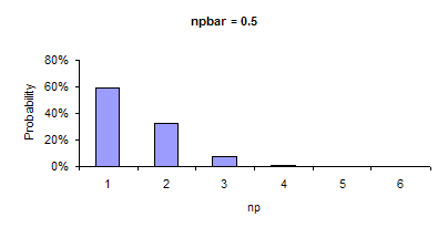
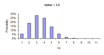
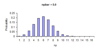
If n*pbar is not sufficiently large, the binomial distribution is not symmetrical. In these cases, the control limit equations are no longer valid. n*pbar is not sufficiently large if n*pbar < 5 or if n*(1-pbar) < 5. This is referred to as small sample case for p and np charts. The figures below demonstrate how the shape of the binomial distribution changes as n*pbar changes from 0.5 to 5.0. As can be seen in the figures, the binomial distribution becomes more symmetrical and approaches the shape of a normal distribution as n*pbar becomes larger. When the distribution is symmetrical, the control limit equations are valid.
Small Sample Case
If n*pbar < 5 or if n*(1-pbar) < 5, the above control limit equations cannot be used to determine the control limits. The control limits must be derived from the binomial distribution. We have generated a table that gives you the control limits in this small sample case. The table is available for download from the website at this link (small sample case p and np charts download).
The table gives the upper and lower control limits for various values of pbar from 0.001 to 0.5 and for values of n from 5 to 50. These control limits are exact solutions of the equation governing the binomial distribution with the assumption that the probability (P) of obtaining a point beyond the control limits is less than or equal to 0.003:
P(p <= LCLp) + P(p >= UCLp) <= 0.003
The limits given in the table are for np charts for various values of p and n. To obtain the limits for a p chart or convert np to p, use the following relationships:
UCLp = UCLnp/n
LCLp = LCLnp/n
pbar = n*pbar/n
To understand how to use the table and how it was developed, consider the following example. Suppose you are sampling 10 items (such as invoices or expense accounts) on a regular basis. The average fraction defective has been determined to be 0.01. Thus:
n*pbar= (10)(0.01) = 0.1
Since n*pbar < 5, the table must be used to determine the control limits. The table gives the control limits for the np chart. The control limits from the table for p = 0.01 and n = 10 are:
UCLnp = 3
LCLnp = None
A portion of the table is shown below.
| n | 8 |
9 |
10 |
|||
| pbar | LCL | UCL |
LCL | UCL | LCL | UCL |
| 0.01 | – | 2 | – | 3 | – | 3 |
| 0.02 | – | 3 | – | 3 | – | 3 |
| 0.03 | – | 3 | – | 3 | – | 3 |
| 0.04 | – | 4 | – | 4 | – | 4 |
| 0.05 | – | 4 | – | 4 | – | 4 |
| 0.06 | – | 4 | – | 4 | – | 4 |
| 0.07 | – | 4 | – | 4 | – | 5 |
| 0.08 | – | 4 | – | 5 | – | 5 |
| 0.09 | – | 5 | – | 5 | – | 5 |
| 0.10 | – | 5 | – | 5 | – | 5 |
| 0.11 | – | 5 | – | 5 | – | 5 |
| 0.12 | – | 5 | – | 5 | – | 6 |
| 0.13 | – | 5 | – | 5 | – | 6 |
| 0.14 | – | 5 | – | 6 | – | 6 |
| 0.15 | – | 5 | – | 6 | – | 6 |
| 0.16 | – | 6 | – | 6 | – | 6 |
| 0.17 | – | 6 | – | 6 | – | 6 |
| 0.18 | – | 6 | – | 6 | – | 7 |
| 0.19 | – | 6 | – | 6 | – | 7 |
| 0.20 | – | 6 | – | 7 | – | 7 |
The control limits are converted from an np chart to a p chart by dividing by n:
UCLp = UCLnp/n = 3/10 = 0.3
LCLp = LCLnp/n = None/10 = None
If the control limit equations were used, the control limits would be:
The LCLp is actually -0.08 but since it is less than zero, there is no LCLp. Note the difference between the UCLp calculated using the equations (UCLp = 0.1) and that obtained from the table (UCLp = 0.3). This difference is simply due to the fact that, when npbar < 5, the binomial distribution is no longer symmetrical. The control limit equations no longer provide the same probability as when npbar > 5.
The control limits in the table were obtained from the equation governing the binomial distribution. In Microsoft Excel, you can use the function “Binomdist” to determine this. For this example, the probability of finding 0, 1, 2, and 3 defective items in the sample size of 10 with npbar = 0.01 can be calculated. The calculation results are summarized below.
| Number Defective |
Probability |
| 0 | 0.904 |
| 1 | 0.091 |
| 2 | 0.004 |
| 3 | 0.0001 |
The probability of the sample containing 0 defective items is 904 out of 1,000. The probability of the sample containing 0 or 1 defective item is 995 out of 1,000. The probability of the sample containing 0, 1, or 2 defective items is 999 out of 1,000. The control limits in the table are determined so that the probability of obtaining a point beyond the control limits is less than or equal to 0.003 (or 3 out of 1,000). For this case, the probability becomes less than 0.003 when the number of defective items is 3 or more. Thus, the upper control limit for this example is 3.
The table does go beyond n*pbar < 5. It has values of n to 50 and pbar to 0.5 For n = 50 and pbar = 0.5, the table gives the following limits for the np chart:
LCLnp = 14
UCLnp = 36
Note that n*pbar = 25 in this case. The control limit equations for the np chart give the following results:
UCLnp = 35.6
LCLnp = 14.3
When n*pbar is large enough, the control limit equations are valid.
Summary
The p and np chart are used to monitor variation in yes/no type data. The control limit equations are valid as long as n*pbar > 5 or n*(1-pbar) > 5. If this is not true, the binomial distribution which governs the p and np control charts is not symmetrical. This is called the small sample case for the p and np control charts. In the case when n*pbar < 5 or n*(1-pbar) < 5, the actual binomial distribution must be used. A table has been provided for pbar = .001 to .5 and n from 4 to 50 that provides these control limits.


