How Many Samples Do I Need?

June 2015

We are always trying to improve things – our processes at work, our health, our children’s test scores – the list goes on and on. But how do we decide if something we do has made a real difference? For example, how do we know if:

• A new process produces a product with the same hardness as the old process?
• The raw material density from a new supplier is the same as the old supplier?
• A drug has decreased your blood pressure?
• A new teaching method has impacted test scores?

Only one way I know. And that is to use data. No matter where you work, you need data of some type to make a decision. But rarely can you do 100% inspection. Costs too much, takes too long, uses up all the product. So, you must take samples – and that generates the following question:

How many samples do I need to make a good decision?

Such a simple, straightforward question. Correct? How many samples do you need to determine if the new process makes a product with the same hardness as the old process? 1? 5? 10? 30? That value of 30 is used a lot – must be a good sample size. Right?

Answering the question of “how many samples do I need” is easy. Just pick a number, like 30. Understanding the impact of that number you pick is not quite so easy. This month’s newsletter takes a look at how to determine the sample size you need to make decisions about your process. It is all about “power” and about the potential for making errors.

In this issue:

• Hypothesis Testing Review
• The Difference to Detect
• Type 1 and 2 Errors and Power
• Type 1 and Type 2 Errors: A Visual Look
• Determining the Number of Samples You Need
• Power Curves
• Summary
• Quick Links

You may download a pdf copy of this publication at this link. Please feel free to leave a comment at the end of the publication.

Hypothesis Testing Review

Last month’s publication took a look at the steps in hypothesis testing. We will build upon that foundation in this publication. The example used in that publication is that a lean six sigma project team is recommending a change in the coating process to help reduce costs.

The thickness of the coating is a key variable in the process. The average coating thickness is 5 mil. The team wants to be sure that the coating thickness remains the same before the process change is approved. The team performs a hypothesis test to prove that the average coating thickness will not change.

The null hypothesis (H0) is that the process change will not impact the average coating thickness, i.e., the average coating thickness (μ) will remain at 5. This is written as:

H₀ = 5

The alternative hypothesis is that the process change will have an effect on the average coating thickness and the average coating thickness will not equal 5. This is written as:

H₁≠ 5

This is called a two-sided hypothesis test since you are only interested if the mean is not equal to 5. You can have one-sided tests where you want the mean to be greater than or less than some value.

The team picked α = 0.05 as the significance level.1 – α gives us the confidence level. With α = 0.05, our confidence level is 95%.α also represents the probability of rejecting the null hypothesis when it is actually true. This is called a Type 1 error. More on this below.

The team made the process change, took 25 samples and measured the coating thickness. They calculated the average and standard deviation of the 25 samples with the following results:

X= average coating thickness = 5.06

s = standard deviation of the coating thickness = 0.20

Now, we can construct a confidence interval around the sample average based on these results. A confidence interval contains the range of values where the true mean will lie. If the hypothesized mean is contained in that confidence interval, we accept the null hypothesis as true. If the hypothesized mean is not contained in the confidence interval, we reject the null hypothesis.

We will assume that we are dealing with a normal distribution. As shown in last month’s publication, z is defined as:

whereX is our sample average, s is standard deviation and n is the sample size.

The confidence interval depends on three things: the significance level (α), the sample size, and the standard deviation. The equation for the confidence interval around a mean is below.

where z_α/2is the standard normal distribution z score with a tail area of α/2. Using α = 0.05 and z_α/2= 1.96, we can calculate the confidence interval:

5.06 – 0.0784 ≤ μ ≤ 5.06 + 0.0784

4.9816 ≤ μ ≤ 5.1384

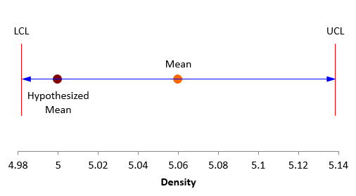
We say then that we can be 95% confident that the truemean of the coating is between 4.9816 (the lower confidence limit) and 5.1384 (the upper confidence limit). Since 5 is included in this interval, we conclude that the null hypothesis is true. This is shown in Figure 1

Figure 1: Confidence Limit for Coating Results

We could also determine a p value based on the data and use this to determine if we accept the null hypothesis as we did in last month’s publication. The calculated p value is 0.1336, which is greater than 0.05 (our value of α), so we conclude that the null hypothesis is true.

The Difference to Detect

One question that is often ignored in these types of studies is:

What is the difference you want to be able to detect?

The team wants to be sure that the average coating is not different than 5. But with a new process, the average will most likely not remain identical – there will be a change no matter how slight. So, the question becomes how far from 5 can the new process average be and still be acceptable. This is the difference you want to be able to detect. We will call this difference δ. The confidence interval equation above can be rewritten as:

X-δ ≤ μ ≤X+δ

where

As shown in the confidence interval calculation above, δ = 0.0784. What does this mean? It means that, for the 25 samples the team took, they could detect a difference in the coating mean as long as it was greater than ±0.0784. Differences less than that could not be detected.

Suppose it was critical to be able to detect a difference of δ = ±0.05. This value is less than 0.0784. So, we have to decrease δ. There are three ways to decreaseδ based on the equation above:

• Increase α, the significance level (which makes z_α/2smaller)
• Decrease the standard deviation
• Increase the sample size

Most of the time, we like using 95% confidence level so we don’t want to change α. We don’t really want to increase the chance of a Type 1 error – rejecting the null hypothesis when it true. Not much we can do about the standard deviation in the short term. So, we need to increase the sample size. But by how much?

You can solve the above equation for n to estimate how many samples you to detect a change of δ.

You would need 62 samples to be able to detect a difference of 0.05. Now we have our number of samples we need to detect a difference of 0.05. And we have an equation for find the number of samples we need to detect the difference we want to detect – at least for the normal distribution. Are we done now? Not quite.

Type 1 and 2 Errors and Power

In the coating example, the null hypothesis (Ho) is that the true mean = 5: The alternative hypothesis (H1) is that the true mean does not equal 5: One of these must be true. We do not in reality which is true and which false. That is why we take the samples and do the calculations. But with sampling, there is always the chance of making an error.

For example, suppose that the reality is that the null hypothesis is true – the true mean is equal to 5. Based on our sampling results, we can either decide that the null hypothesis is true or it is false. If based on our sampling, we decide that the null hypothesis is true, then we are correct. But if we decide, based on our sampling, that it is false, then we have rejected the null hypothesis when it is actually true. This is an error and is called a Type 1 error as we stated before. It is denoted by α.

But there is a flip side to this. Suppose that the reality is that the null hypothesis is false – the true mean does not equal 5. If, based on our sampling, we conclude that the null hypothesis is false, then we are correct – we made the right decision. However, if based on our sampling, we conclude that the null hypothesis is true, then we are making an error. We are saying the null hypothesis is true when in reality it is false. This is called a Type 2 error and is denoted by β. We often don’t take into this type of error.

The possible outcomes from our sampling are shown in the table below. We want to make errors as seldom as possible – so we want to minimize how often we make Type 1 errors (that is we want α to be small) and how often we make Type 2 errors (that is we wantβ to be small).

Table 1: Type 1 and Type 2 Errors

		Conclusion from Sampling
		H0 is True	H0 is False
Reality	H0 is True	Correct	Type 1 Error (α)
	H0 is False	Type Two Error( β)	Correct

Power is directly related to β. Power is defined as:

Power = 1 – β

When someone says the sampling scheme has a power of 80%, it means that there is a 20% of making a Type 2 error – accepting the null hypothesis as true when it is in fact false.

Type 1 and Type 2 Errors: A Visual Look

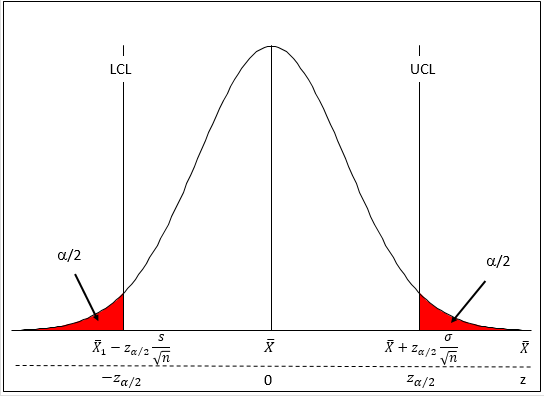
It helps to visualize the two types of errors to help us understand what they mean. Figure 2 shows the Type 1 error for a two-sided test like in the coating thickness example. One x-axis is based on the distribution of sample averages; the other on the z value (average = 0; standard deviation = 1).

Figure 2: Type 1 Error

As long as the hypothesized mean (μ₀) is between the lower confidence limit (LCL) and upper confidence limit (UCL), we accept the null hypothesis. This is what we did in the coating thickness example and as shown in Figure 1. You control how often you make a Type 1 error through the selection of α.

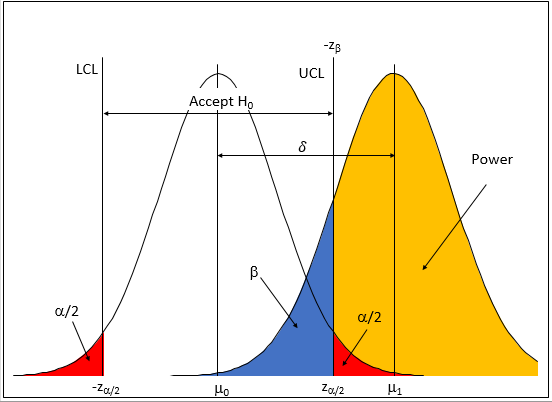
Now suppose that the true mean has shifted from μ₀to μ₁= μ₀+ δ. Figure 3 shows this additional distribution in addition to the distribution in Figure 2.

Figure 3: Type 1 and 2 Errors

Look at the “Accept H₀” range in the figure. This is the range where we will accept that the null hypothesis is true – because we are assuming that our process distribution is on the left side of Figure 3. In our coating thickness example, it is the distribution related to H₀= 5.

But suppose that the process change really did move the true mean byδso H₀≠ 5 is really true. We are now sampling from the distribution on the right. If we sample that distribution and get a result that falls into the blue area of that distribution, we would conclude that the null hypothesis is true – when in fact it is false. So, we would make a Type 2 error. The value where this occurs is –z_βas shown in Figure 3.

The “power” is shown in the yellow shaded portion of Figure 3. If our sample result is in this area, we conclude correctly and reject the null hypothesis in favor of the alternate hypothesis. You want power to large – 80% or more. Power is always related to the difference you want to detect. It has no meaning without a difference to detect.

 

Determining the Number of Samples You Need

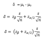
Take a look at Figure 3. Note that there are two ways to define the upper confidence limit:

You can now solve for δ using the two above equations:

You can use this equation to determine what difference you can detect (for a normal distribution) for values of α, β, s and n.

You can also solve the above equation for n:

You can use this equation to solve for the number of samples you need for given values of α, β, s and δ. Return to the coating thickness example. Suppose it was important that you could detect a difference down to 0.05 with a power of 90% (β= 0.10), α= 0.05, and s = 0.2. How many samples do you need? Using z_α/2= 1.96 and z_β= 1.282:

You would need 169 samples to have a 10% of chance of accepting the null hypothesis when it is in fact false and a 5% chance of rejecting the null hypothesis when it is in fact true. Note that is a lot more than the 25 samples the team took to determine if the null hypothesis was true.

What is the power if we want to detect a difference of δ =0.05 and take 25 samples? As it turns out the power is about 24%. This means that you have a 76% chance of making a Type 2 error – accepting the null hypothesis when it is in fact false. That is why it is important to determine the difference you want to detect as well as the values to use forα and β.

Power Curves

Many software packages (including SPC for Excel) will generate power curves for sampling plans. An estimate of the standard deviation is needed. Two of the following three must be entered: the sample size, the difference to detect, and the power. Alpha and the type of test (two-sided or one-sided) are also required.

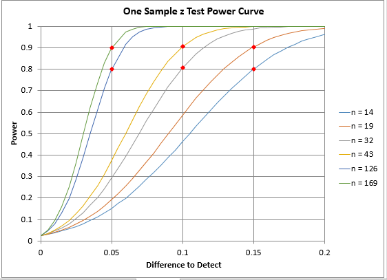
Return to the coating thickness issue. Suppose we wanted to know the sample size required to detect differences of 0.15, 0.10 and 0.05 at a power of 80% and 90% using a standard deviation of 0.2 with alpha = 0.05 and a two-sided test. The power curve in Figure 4 was generated using the SPC for Excel software. To see a video of power curves in SPC for Excel, click here.

Figure 4: Power Curve Example

The table below summarizes the results. It requires 14 samples to detect a difference of 0.15 with a power of 80% and 19 samples for a power of 90%. To detect a difference of 0.05 at 80% power requires 126 samples and 169 samples at 90% power. The actual power column represents a calculation of the actual power since the sample size is rounded.

Table 2: Power Curve Results

Difference to Detect	Sample Size	Power	Actual Power
0.15	14	0.8	0.801
0.15	19	0.9	0.905
0.1	32	0.8	0.807
0.1	43	0.9	0.906
0.05	126	0.8	0.801
0.05	169	0.9	0.901

Quite often, you will be surprised at how many samples you need to take to reach a good power number. The power curves help you make decisions about the tradeoff between sample size, difference to detect, and power.SummaryThis publication examined how to determine how many samples you need to take to make a decision about your process. Far too often we only worry about Type 1 errors, when in reality, we need to be concerned also with Type 2 errors. You will often need to take tradeoffs to reduce the sample size needed – tradeoffs in terms of the difference to detect or the power – as well as the probability of making a Type 1 error. Deciding on the difference you want to detect should be done before worrying about how many samples you need.

Summary

This publication examined how to determine how many samples you need to take to make a decision about your process. Far too often we only worry about Type 1 errors, when in reality, we need to be concerned also with Type 2 errors. You will often need to take tradeoffs to reduce the sample size needed – tradeoffs in terms of the difference to detect or the power – as well as the probability of making a Type 1 error. Deciding on the difference you want to detect should be done before worrying about how many samples you need.