May 2009
In this issue:
- Introduction to the Normal Distribution
- Probability Density Function
- Standard Normal Distribution
- How to Use the Normal Distribution
- Normal Distribution and Specifications
- Quick Links
Introduction to the Normal Distribution
If you search for “normal distribution” on Google, you will get a lot of hits. Wikipedia, the free encyclopedia, starts out its normal distribution with:
“In probability theory and statistics, the normal distribution or Gaussian distribution is a continuous probability distribution that describes data that clusters around a mean or average. The graph of the associated probability density function is bell-shaped, with a peak at the mean, and is known as the Gaussian function or bell curve.”
So, what does this mean to us and how do we use normal distributions? This month’s newsletter examines the normal distribution.
The normal distribution is shown below. It is shaped like a bell
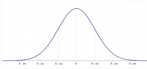
The normal distribution has several interesting characteristics:
- The shape of the distribution is determined by the average, μ (orX), and the standard deviation, σ.
- The highest point on the curve is the average.
- The distribution is symmetrical about the average.
- As you move away from the average, the points occur with less frequency.
- Most of the area under the curve (99.7%) lies between -3σ and +3σ of the average.
Probability Density Function
The probability density function for the normal distribution is given by:
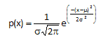
where x is some value between -∞ to +∞, μ is the average and σ is the standard deviation. The standard deviation is an indication of how wide the normal distribution is. The average gives the location of the normal distribution.
The distributions below show how the normal distribution changes as the standard deviation changes. The average is 100 and there are three different distributions with standard deviations of 5, 10, and 20. Note that the larger the standard deviation, the wider the distribution. When you are making a control chart, the range chart is actually monitoring the “width” of the distribution. The range chart answers the following question: is the spread in my data staying the same over time (in control) or is the spread getting smaller or larger (out of control)?
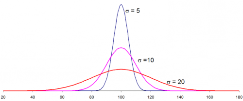
The distributions above were generated using Excel’s NORMSDIST function using an average of 100, one of the three standard deviations above and an X values range from 20 to 180. So, if you know your process average and process standard deviation, you can easily draw the normal distribution for your process. This, of course, assumes that your process is normally distributed.
Standard Normal Distribution
For an average of 0 and a standard deviation of 1, the formula above becomes:
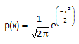
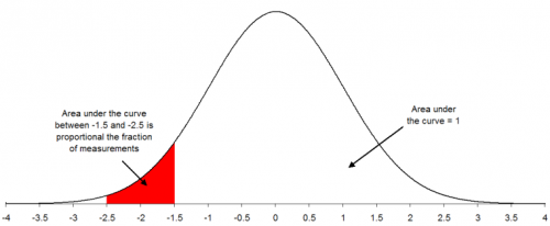
This is known as the standard normal distribution. For this distribution, the area under the curve from -∞ to +∞ is equal to 1.0. In addition, the area under the curve is proportional to the fraction of measurements that fall in that region. These two facts will be used to help determine the fraction of measurements that fall above some value (such as a specification limit), below some value, or between two values. The standard normal distribution is shown below.
How to Use the Normal Distribution
Suppose you are interested in a certain quality characteristic, X. You have been monitoring this characteristic using an X-R chart. Both the X chart and the range chart are in statistical control. This means that you can predict what your process will make in the near future. You also know that you have good estimates of the process average (from the X chart) and the process standard deviation (from the range chart). Suppose that X = 100 and that σ = 10.
In addition, you have constructed a histogram for the last month’s data. The histogram is shown below.
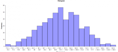
This histogram appears to be bell-shaped so you assume that you are dealing with a normal distribution. You can then draw the normal distribution for this process because you know the average and standard deviation (from your control charts). The normal distribution for this process is shown below.
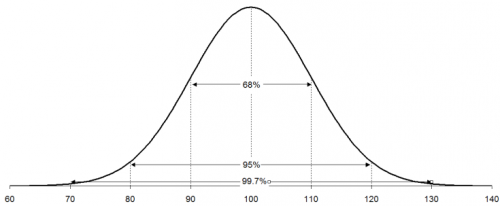
A normal distribution has the following properties:
- 68% of the data is within +/- 1 standard deviation of the average
- 95% of the data is within +/- 2 standard deviations of the average
- 99.7% of the data is within +/- 3 standard deviations of the average
For your process, the following calculations can be done:
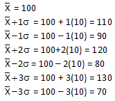
Thus, 68% of the data lies between 90 and 110; 95% of the data between 80 and 120; and 99.7% of the data between 70 and 130. The specifications for the process have been 65 to 140. Life is good – everything has been within specifications.
Normal Distribution and Specifications
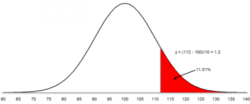
Now suppose a customer has decided that the upper specification limit for your process should be 112. You can easily see from the histogram and the normal distribution that some of your product will be out of specification. The question is how much will be out of specification. This is where the z value becomes important. z is defined by the equation:

For our example, x = 112, so
z = (112-100)/10 = 12/10 = 1.2
z represents the number of standard deviations some value is away from the average. So, 112 is 1.2 standard deviations above the average. If z is negative, it means that the value is below the average.
To find out how much product is more than 1.2 standard deviations above the average, you can use what is called the “z table.” The z table gives the fraction of process output that is beyond some value x that is z standard deviations from the average. The z table is given below.
z Table: Standard Normal Distribution
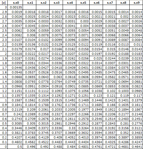
The table above returns a value of .1151 for a value of z = 1.2. This means that 11.51% of the data will be above the upper specification limit of 112. This is shown in the figure below. The area in red represents material that is out of specifications on the high side.
You can also use the NORMSDIST function in Excel to find the above result. This function in Excel returns the fraction of results less than a value. So, you must use 1 – NORMSDIST(z) if you want the fraction of data above z. In this example: 1- NORMSDIST(1.2) = .11507
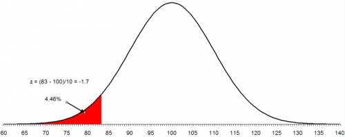
To make matters worse, the customer has now set the lower specification as 83. You want to find out what percent of the product will be out of specification on the low side. The process is the same as above. In this case:
z = (83 – 100)/10 = -17/10 = -1.7
This means that 83 is 1.7 standard deviations below the average. From the z tables, the fraction of data below 1.7 is 0.0446 or 4.46%. In Excel, NORMSDIST(-1.7) = 0.044565. The figure below shows this situation. The area in red represents the product that is below the lower specification limit.
To find out the area between two values, you use the fact that the area under the standard normal curve is 1. For example, suppose you want to find out the area between 83 and 112. We know that the area below 83 is .0446 and the area above 112 is .1151. Then the area between 83 and 112 is given by:
1 – .0446 – .1151 = 0.8403
Thus, 84.03% of the data lies between 83 and 112. Thus, with the new specifications, 84% of your product will be within specification. The remaining 16% will be out specification. And since the process is in statistical control, this will continue to be true until the process is changed fundamentally.