October 2010
If you live in the United States, you are keenly aware that the mid-term elections are this Tuesday, November 2, 2010. Watch TV – and every other commercial is a political ad. Listen to the radio – almost every ad is a political ad. Watch the news and they give you the latest poll results – candidate A was 2 points behind candidate B, but the latest poll shows that candidate A is now 3 points up! But, the margin of error is plus or minus 4%. What do these poll numbers mean? This newsletter takes a look at how these numbers are determined and what they mean.
In this issue:
- The Math
- Example: Polls
- What Does 95% Confidence Mean?
- Example: Football Quarterback
- What Sample Size Do I Need?
- Sample Size Example
- Summary
- Quick Links
For example, consider the race for the Nevada senator. The incumbent is Senate Majority Leader Harry Reid. His opponent is Republican Sharron Angle. The following is from Rasmussen Reports on October 26, 2010
“The latest Rasmussen Reports telephone survey of Likely Voters in Nevada finds Angle with 49% support to Reid’s 45%. Four percent (4%) like some other candidate in the race, and two percent (2%) remain undecided with one week until Election Day.”
and
“The survey of 750 Likely Voters in Nevada was conducted on October 25, 2010 by Rasmussen Reports. The margin of sampling error is ± 4 percentage points with a 95% level of confidence.”
What does this really mean?
The Math
In this newsletter, we will consider the simplest case. We want to do what proportion (fraction) of a population possesses a certain attribute. For example, we might want to find out the proportion of people in a certain state favor a certain candidate, favor gun control, or favor government-sponsored health care. One method we could use is to ask each and every person in the state if they favor the topic. This, of course, would take while and would be very expensive. But we would know the true proportion because we talked to everyone.
This is where inference comes in. Inference is the process of drawing conclusions about a parameter one is seeking to measure or estimate from a limited amount of data. We do this by taking samples from the population. We then used the sample results to estimate the parameter in which we are interested. Because it is a sample, it is estimate of the true value of the parameter. And this estimate has some error associated with it. Let’s see how this works.
A random variable that can take on only two values is called a Bernoulli random variable. That is the case we are considering. Each person in the population is either for or against the topic. This type of binary data, which indicates the presence or absence of a certain attribute, are often modeled as a random sample from the Bernoulli distribution with parameter p, where p is the portion of the population possessing the attribute (reference: Statistics and Data Analysis by A. Tamhane and D. Dunlop).
Suppose you have a large population and you want to estimate p. You take a random sample (Xi) of size n from the population. If the Xi has the attribute, then Xi = 1. If the Xi does not have the attribute then Xi = 0. The probability that Xi = 1 is p. The probability that Xi = 0 is 1 – p. If Y = the sum of the Xi, then an estimate of p can be found from the sample proportion:
![]()
It turns out that if the sample size n is large enough, p will be a normal distribution with an average of p and variance of pq/n where q = 1 – p. This is due to the Central Limit Theorem. n is consider if np ≥ 10 and n(1-p) ≥ 10.
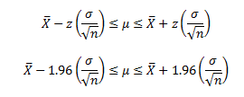
Under these conditions, we can use the equations for confidence interval around a mean to develop a confidence interval around p. If a random sample is taken from a normal distribution, the z value for the sample mean is defined as follows:
![]()
where X = the sample average, m = population average (the parameter of interest), s = the variance, and n = the sample size. Rearranging this gives:
![]()
For 95% confidence, z = -1.96 or z = 1.96, so
Now we can insert p as the average and pq/n as the variance.
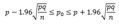
where po = population proportion with the attribute. We can now use this equation for our 95% confidence interval.
Example: Polls
Let’s take a look at the race between Reid and Angle. The Rasmussen poll of 750 likely voters had 49% favoring Angle with a margin of error of ±4%. We can apply the above to determine the confidence interval for those that favor Angle. Rasmussen’s sample is from the population of “likely voters” in the state of Nevada. In this example, p = 0.49. So, q = 1 – 0.49 = 0.51.
The confidence interval is then:
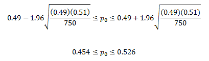
Thus, the 95% confidence interval for the % of likely voters who favor Angle is 45.4% to 52.6%. This is a range of 7.2% so it is said that the results are ±3.6%. Note that this is different than the ± 4% from the Rasmussen poll. The math is different when you consider more than binary results – which they do since they are considering more than two candidates and whether the person has decided for whom they will vote.
What Does 95% Confidence Mean?
What does the confidence interval above mean? Does it mean that we 95% certain that the value of p0 lies between 45.4% and 52.6%? No, this is not how you interpret a confidence interval. In this case, p0 is unknown. Since it is unknown, we can’t know for sure if it is in that interval. What the 95% means is, if we take an infinite number of samples of size n from the population and calculate the confidence interval, 95% of these confidence intervals will contain p0.
Example: Football Quarterback
Kellen Moore is the quarterback for the Boise State Broncos in college football. Through October 26th of this year, he is the highest ranked quarterback in the nation. This year-to-date, he has completed 125 out of 179 passes or 69.8% of his passes. Last year he completed 277 passes out 431 or 64.3% of his passes. Question: is his pass completion percentage significantly better than last year’s completion percentage?
In this example, p = 0.698, q = 1 – p = 0.302, and n = 179.
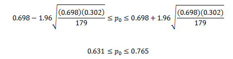
Thus, the 95% confidence interval for Moore’s passing completion this year is 63.1% to 76.5%. This gives a margin of error of ± 6.7%.
How can we decrease the margin of error? Only one way to do that and that is to increase the sample size.
What Sample Size Do I Need?
Your sample size depends on what you want to accomplish. From the equation for the confidence limit around p, let E be the margin of error:
![]()
Solve that for n.
![]()
If you have a prior estimate of p, then you can use this estimate in the equation. However, if you do not, then you can take the conservative approach and set p = q = 0.50.
Sample Size Example
Suppose I want to find out what percent of American voters support President Obama’s health care plan. I want the margin of error to be ± 3% with a 95% confidence. I don’t have a prior estimate so I will use p = q = 0.5. Under these conditions, z = 1.96, E = 3% = 0.03. The sample size I need is then given by:
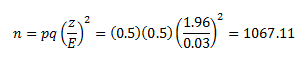
Rounding up means that I would need to survey 1,068 voters. Now suppose I want the margin of error to be ± 1%. In this case,
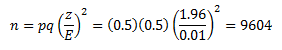
You can see that the sample size increases a lot as the margin error decreases. This is due to the fact that the margin of error is in the denominator of the squared term.
Summary
This newsletter has examined how you can determine the sample size you need to determine what percent of a population has a certain attribute within a given margin of error. It is important the sample taken from the population be random – which means that each member of the population has the same opportunity to be sampled.