February 2006
In this issue:
Statistical control, stability, consistent and predictable. What do these terms mean? Are they really important to us? The answer is yes! And it has an impact on you if you ever do any of the following:
- Calculate an average and standard deviation from a set of data
- Calculate a Cpk for a process
- Use hypothesis testing and confidence intervals
- Compare this month’s financial results to budget or to last year’s results
Basically, if you use statistics for analysis, the concepts of statistical control and stability are very important. Many people do these things on a regular basis. But none of the above statistics have any meaning unless the process that generates them is stable – in control. A reader from last month’s e-zine on histograms reminded me that I should have emphasized this point. Using a histogram for decision making and data analysis is good – but only if the process that generated the histogram is consistent over time. And how do we know that? Only through control charts.
How do control charts work and why are they important? The answers to these questions really affect how well you use data. This month’s e-zine takes an in-depth look at how a control chart works and why the control chart is an invaluable tool.
The Five Questions
 Suppose you have just been put in charge of a bagging operation. The process involves putting sand into bags. The target for the bag weight is 50 pounds with a tolerance of +/- 2 pounds. You understand that there have been concerns about the variability in the bag weights. You want to understand what this variability is and determine how to reduce it. How would you go about that? What are some of the questions you might want to answer?
Five good questions are:
- What is the average bag weight?
- How much variation is there about the average?
- What does the shape of that variation look like?
- Does the average and variation stay the same over time?
- How do the individual bag weights compare to specifications?
The keywords in the questions above are “stay the same over time.” You can do any of the calculations above – find the average, the standard deviation, construct a histogram, calculate the Cpk value. But none of these have any meaning unless your process is stable – in statistical control.
A quick refresher on variation before answering these questions. Processes, whether manufacturing or service in nature, are variable. You won’t always get the same result each time. The reason for this is that there are sources of variation in all processes. There are two major sources of variation. One is common cause variation. It is the variation which is inherent in the process due to the way it was designed and is managed daily. Common cause variation can be reduced. To reduce common cause variation, the system must be changed. This is normally management’s responsibility. There will always be common cause variation present in a process. Think about the time it takes you to get to work. There is a certain amount of “normal” variation in this process. Maybe it takes you anywhere from 30 to 40 minutes. This is common cause of variation. It is consistent and predictable.
The second type of variation is special cause variation. This variation is caused by things that don’t normally happen in the process. Those closest to the process have the responsibility for finding and removing special causes of variation (although some require the input of management). If a process has special causes, it is not stable. For example, if you have a flat tire on the way to work, it will take you longer to get to work than “normal.” Special causes of variation cannot be predicted, and they prevent your process from being consistent and predictable.
A process is in statistical control if only common cause variation is present. How do we know if only common cause variation is present or if there are also special causes of variation present? The only way to determine this is through the use of a control chart. For more information on variation, please see the January 2004 e-zine that is available on our website. Now on to answering the five questions.
The Average
Let’s start with the first question: the average bag weight. In reality, you can’t know what the true average bag weight is from the process. You can only estimate this average. This true average is called the population average. So, how can you estimate the population average?
You could start by going to the process and weighing one bag. Suppose this bag weighs 50.1 pounds. Is this a good estimate of the population average? You probably will not think taking one sample is a very good method of estimating the average. Obviously, you will need more samples.
You decide to take 5 bags and calculate the average weight of those five bags as shown below.
(50.1 + 50.9 +50.8 + 50.1 + 49.6)/5 = 50.3
This average is 50.3. Is that a better estimate of the population average? It is better than the one bag weight. But, how comfortable are you saying that with just five bag weights, you have a good estimate of that population average? Again, probably not that comfortable.
But suppose you decide to continue this process. Each hour you take 5 bags and weigh them. These 5 bags that are taken each hour are called a subgroup. The average you calculate is called the subgroup average.
The data you have for the first 20 hours are given below. The average is given along with the range, which we will use later when we discuss variation of individual results.
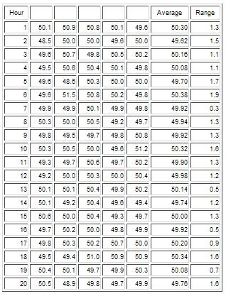
The averages are not the same for each set of 5 bags. The average seems to bounce around. The average of these 100 bag is 50.02. With this many samples, you might feel that this is a good estimate of what the bagging processes produces – that 50.02 is a good estimate of the unknown population average. But, in reality, you don’t know this yet because you have not addressed the issue of statistical control. An average has no meaning unless the process is consistent and predictable.
The Average Over Time
 To discover if the average is valid, you can plot the subgroup averages over time as shown in the figure. A subgroup average is designated by Xbar. This plot shows the variation between subgroup averages – i.e., how the subgroup averages vary over time. There is some variation in the results as expected, but now you can see what the variation looks like.
You can further quantify this variation by adding an average line and control limits. The average is simply the average of the subgroup averages and is referred to as “X double bar”. This is 50.02. You can also add “control limits.” These control limits are determined from the data. Using the data, we compute a range of values we would expect if only common cause variation is present. The largest number we would expect is called the upper control limit (UCL). The smallest number we would expect is called the lower control limit (LCL). The calculations depend on the type of control chart (see the past e-zines on the website for the calculations for various types of control charts). The average and control limits are given in the chart above. This chart is called the Xbar chart.
In general, if all the results fall between LCL and the UCL and there is no evidence of nonrandom patterns, the process is in statistical control, i.e., only common cause variation is present. This means the bagging process is consistent and predictable. You know what it will do (and not do) in the future. In this example, a bag of sand will weigh between 49.33 and 50.71 with a long term average of 50.02. And since there are only common causes of variation present, this will not change as long as the process stays the same.
So, we have answered question 1 using the Xbar chart. Our estimate of the population average is 50.02. In addition, we have answered part of question 4. This average will not change as long as the process stays the same and there are no special causes of variation. Special causes of variation could include new operators, different sand supplier, etc.
The Variation Around the Average
Question 2 asked how much variation there is about the average – i.e., how much do the individual values vary about this average? This question is essentially asking what the standard deviation of the process is. The standard deviation measures how much the individual results vary about an average (see our August 2005 e-zine: Explaining the Standard Deviation).
To determine this, you can use the range values that are given in the table above. For each of the 5 bag weights, you determine the subgroup average. You can also calculate a range value for each subgroup. The range is simply the maximum value – minimum value. For the first subgroup, the range is
R = 50.9 – 49.6 = 1.3
This range value is a measure of the variation between individual values – the maximum and the minimum.
The Range Over Time
 You can plot the range values over time. The range values are shown in this figure. This chart shows the within subgroup variation and how that varies from subgroup to subgroup. You can enhance this chart by adding the average range (called Rbar) and the control limits.
In this example, the range only has an UCL. Again, since there are no patterns and no points beyond the control limits, the process just has common causes of variation present. It is consistent and predicable. This means the variation in the individual values about the average is the same over time.
You can estimate the standard deviation from the average range using an equation that depends on the subgroup size (see our March 2005 e-zine on Xbar-R charts for more information). The standard deviation is 0.512 based on the average range. This is our estimate of the population standard deviation – the true variation in the individual values about the average. And since the process is in control, the standard deviation will stay the same over time as long as the process does not change and there are no special causes of variation.
So, we have answered question 2 using the range chart. The variation in individual values is 0.512, the estimate of the population standard deviation. We have also answered the last part of question 4. This variation will not change as long as the process stays the same and there are no special causes introduced. Remember, a standard deviation has no meaning unless the process is consistent and predictable (in control).
The Shape and Specs
 And finally, questions 3 and 5 – what does the shape of the variation look like and how does it compare to specifications? The shape of the variation comes from the histogram (see our December 2005 and January 2006 e-zines on histograms). Comparing to specification is handled using a process capability analysis (see our three part e-zine starting October 2004). The histogram/process capability analysis for this data is shown in the figure. The process is capable of meeting specifications. And since it is in control, it will continue to do so over time until the process changes.
And remember, like the average and the standard deviation, the histogram and value of Cpk have no meaning unless the process is consistent and predictable.
This is why it is so important to understand control charts and statistical control.
Example
 The key point is that the statistics you see day in and day out must be interpreted in the context of the process that generated them. Was that process in control and stable? Or did it have special causes of variation present – flat tires? If it had special causes present, you will not get a similar result next time because you cannot predict what a process with special causes of variation will do in the future.
The chart shown above will produce the same average and the same calculated standard deviation as the first Xbar chart shown on bag weight. But doesn’t it tell a different story? So simple. Just plot the data over time and you will be amazed at what you learn.