November 2009
In this issue:
Introduction
 There is no doubt that accurate and precise measurements are critical for process control and improvement to occur. This month’s newsletter examines how to quickly analyze a measurement system. The method involves the use of control charts to determine if an operator can consistently repeat the measurements and to qualitatively determine if the measurement system can distinguish between samples. It also involves a quantitative method to determine how useful the measurement system is.
Measurement systems with a lot of variability can cause you many problems. Sometimes, there is so much variation in a measurement system that it masks the variation in the process. Suppose you are an engineer. You have determined some process changes that should increase the amount of one component in a process stream. The operating unit makes the process changes and samples are taken to the lab for analysis. Is the measurement system good enough to “see” the improvement caused by the process changes? If not, you will not be able to determine what impact the process changes had. Worse, you may make a wrong judgment about what impact the process changes had. Measurement systems with a lot of variability may mask process improvements.
Sources of Variation
 To illustrate, suppose you are monitoring a process by pulling samples of the product at some regular interval and measuring one critical quality characteristic (X). Obviously, you will not always get the same result when measure for X. Why not? There are many sources of variation in the process. However, these sources can be grouped into three categories:
- variation due to the process itself
- variation due to sampling
- variation due to the measurement system
These three components of variation are related by the following:
![]()
where σt2is the total process variance; σp2is the process variance; σs2is the sampling variance and σms2is the measurement system variance. Note that the relationship is linear in terms of the variance (which is the square of the standard deviation), not the standard deviation.
For our purposes here, we will ignore the variance due to sampling (or more correctly, just include it as part of the process itself). However, for some processes, sampling variation can greatly impact the results. Thus, we will consider the total variance to be:
![]()
Remember geometry? The right triangle? The Pythagorean Theorem? The above equation can be represented by the triangle below.
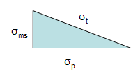
The total standard deviation, σt, for a measurement is equal to the length of the hypotenuse. The process standard deviation, σp, is equal to the length of one side of the triangle and the measurement system standard deviation, σms, is equal to the length of the remaining side.
You can easily see from this triangle what happens as the variation in the product and measurement system changes. If the product standard deviation is larger than the measurement standard deviation, it will have the larger impact on the total standard deviation. However, if the measurement standard deviation becomes too large, it will begin to have the largest impact.
Thus, the objective is to minimize the % variance due to the measurement system:
% Variance due to measurement system = 100(σms2/σt2)
The Procedure
This procedure involves one operator measuring a series of parts or samples more than once using the same measurement system. The steps are shown below.
- Select “p” product samples which reflect the range of production
- Select one operator to perform the measurements
- Randomize the order in which the samples will be run
- Measure each part one time (the operator)
- Randomize the order in which the samples will be run on second time
- Measure each part one time (the operator)
- Analyze the results using an Xbar-R chart
- Determine the % variance due to the measurement system.
There is always the question of how many samples do you need. Usually 10 to 15 is a good number. The larger the sample size, the more confidence you will have in the results. The example below demonstrates the procedure.
Example
To evaluate the measurement system, fifteen polymer samples were taken that accurately reflect the range of production. The inherent viscosity of each sample is the key characteristic. The process inherent viscosity range is 0.60 to 0.95. Each sample was mixed thoroughly and divided in half. Each half of the sample is assumed to be the same in this analysis. One operator then runs each sample in a random order. The samples are labeled in a manner that the operator will not know what sample is being run.
The results are shown in the table below. The first column is the subgroup number. The second column contains the result the operator got the first time the sample was run; the third column contains the results for the second time the sample was run. The next column is the average of the two sample results, while the last column contains the range of the two samples.
| Subgroup | Result 1 | Result 2 | Average | Range |
| S1 | 0.73 | 0.78 | 0.755 | 0.05 |
| S2 | 0.69 | 0.68 | 0.685 | 0.01 |
| S3 | 0.76 | 0.72 | 0.74 | 0.04 |
| S4 | 0.81 | 0.83 | 0.82 | 0.02 |
| S5 | 0.81 | 0.79 | 0.8 | 0.02 |
| S6 | 0.84 | 0.84 | 0.84 | 0 |
| S7 | 0.64 | 0.69 | 0.665 | 0.05 |
| S8 | 0.74 | 0.73 | 0.735 | 0.01 |
| S9 | 0.8 | 0.81 | 0.805 | 0.01 |
| S10 | 0.7 | 0.73 | 0.715 | 0.03 |
| S11 | 0.72 | 0.68 | 0.7 | 0.04 |
| S12 | 0.67 | 0.67 | 0.67 | 0 |
| S13 | 0.66 | 0.67 | 0.665 | 0.01 |
| S14 | 0.7 | 0.72 | 0.71 | 0.02 |
| S15 | 0.71 | 0.69 | 0.7 | 0.02 |
| S16 | 0.64 | 0.62 | 0.63 | 0.02 |
Think about how the data is subgrouped and what sources of variation are present in the average and the range. The first subgroup consists of the two results (0.73 and 0.78) for the sample 1. What causes the variation in these two results? The only differences seen are due to the measurement system because the results are for the same sample. Thus, the ranges are a measure of the variability in the measurement system.
The average for the first sample (0.755) is the average of the two results (0.73 and 0.78). What are the sources of variation in this result? In this case, it is the product as well as the measurement system. Thus, the averages contain both sources of variation, while the range contains only the variation due to the measurement system.
The next step is to analyze the results using an Xbar-R chart with a subgroup size (n) of 2. For more information on Xbar-R chart, please see our March and April 2005 newsletters (see the Articles & Newsletters link to the left). These newsletters show how to construct the control charts including how the control limits are determined.
The range chart is examined first. The range chart, which is monitoring the measurement system variation, is shown below. The average range is 0.0219. The upper control limit for the range chart is 0.0715.
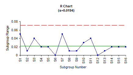
The range chart is in statistical control. This means that the operator is capable of consistently repeating the measurements. If the range chart was out of control, it would mean that the operator is not capable of consistently repeating the measurements. Special causes would be present that should be found and removed.
Since the range chart is in control, we can estimate the measurement system standard deviation. This is given by:
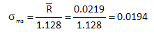
This is the length of measurement system standard deviation leg of the right triangle. The measurement system variance is the square of this number.
σms2= (0.0194)2= 0.000376
The next chart to examine is the Xbar chart. The Xbar chart is shown below. The average is 0.7272. The upper control limit is 0.7683; the lower control limit is 0.6861.
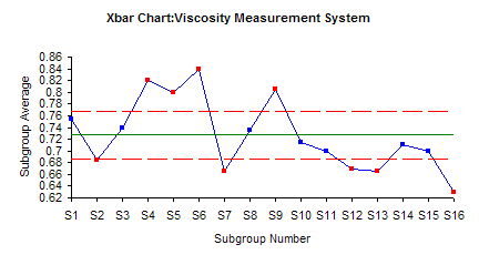
Note that most of the points are out of control (beyond the control limits). Remember the way that the subgroups were formed. The two results from running the same sample were used to form a subgroup. The range is based on the difference in those two results. We would expect this range to be small if the measurement system is precise. The average range is used to calculate the control limits on the Xbar chart:
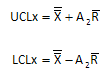
A2 is a control chart constant that depends on subgroup size. The X with the double bar is the overall average. The R with the bar is the average range. Since the average range should be small (assuming the measurement system is precise), the control limits will be narrow compared to the range of subgroup averages plotted. These subgroup averages should be representative of the process variation. In this procedure, you want the points on the Xbar chart to be out of control. If this is the case, the measurement system is capable of distinguishing between samples. The Xbar chart provides a qualitative method of determining how “good” the measurement system is.
In the Xbar chart above, 9 of the 16 points are out of control. The measurement system appears to be able to distinguish between most points. Note that the only out of control test that applies here is points beyond the control limits.
To determine how useful the measurement system is, we now need to compare it to the total variance.
% Variance due to variance method = 100(σms2/σt2)
So, we need to find out what σtis equal to. The best estimate for this would be from a control chart kept on the product characteristic (inherent viscosity in this example). The value of σtwould be estimated from the average range on the range chart for the product.
![]()
where d2 is a control chart constant that depends on subgroup size. This is always the best way to estimate ?t2. Remember that what you are estimating in the equation above is the standard deviation of the individual results. You will need to square it to get the variance.
If you don’t have control chart on the product, you can use the samples in the study as long as they were carefully selected to represent the range of production. In this case, the following equation can be used to estimate σt2.
![]()
The s2 term above is the variance of the subgroup averages. N is the number of times each sample was measured. Using this approach, the variance of the subgroup averages (from the data in the table above) is 0.00386. N is equal to two in this case. So, the total variance is given by:
σt2=0.00386+0.000376/2 = 0.004
We can now calculate the % variance due to the measurement system.
% variance due to measurement system = 100(σms2/ σt2)= 100(0.000376/0.004) = 9.4%
Please note: if the samples don’t reflect the range of production, you will get the wrong estimates for the % of variance due to the measurement system.
The % variance due to the measurement system is 9.4%. Is this good enough? Below is our definition of a precise measurement system:
A precise measurement system is defined as one that is in statistical control with respect to variation (i.e., the range chart) and that is responsible for less than 10% of the total process variance.
Note that this definition has two pieces. First the range chart must be in control when doing the analysis above. In addition, the measurement system variance must be responsible for less than 10% of the total process variance.
Our conclusion in this example is that the measurement system is precise.
Discrimination Ratio
In this excellent book, EMP III: Using Imperfect Data, Dr. Donald Wheeler defines a Discrimination Ratio (DR) to delineate the usefulness of a measurement system. DR is defined as the following:
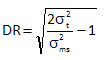
DR ratios above 4 are desirable. You can see from the equation above that DR contains the ratio of the total variance to the measurement system variance. We simply used the inverse of that ratio to say we want the minimum % variance due to the measurement system to be 10%. The table below shows DR as a function of the two ratios
| % Variance Due to Measurement System | Total to MS Variance | DR | % Variance Due to Measurement System | Total to MS Variance | DR | |
| 200.0% | 0.5 | 0.00 | 9.5% | 10.5 | 4.47 | |
| 100.0% | 1 | 1.00 | 9.1% | 11 | 4.58 | |
| 66.7% | 1.5 | 1.41 | 8.7% | 11.5 | 4.69 | |
| 50.0% | 2 | 1.73 | 8.3% | 12 | 4.80 | |
| 40.0% | 2.5 | 2.00 | 8.0% | 12.5 | 4.90 | |
| 33.3% | 3 | 2.24 | 7.7% | 13 | 5.00 | |
| 28.6% | 3.5 | 2.45 | 7.4% | 13.5 | 5.10 | |
| 25.0% | 4 | 2.65 | 7.1% | 14 | 5.20 | |
| 22.2% | 4.5 | 2.83 | 6.9% | 14.5 | 5.29 | |
| 20.0% | 5 | 3.00 | 6.7% | 15 | 5.39 | |
| 18.2% | 5.5 | 3.16 | 6.5% | 15.5 | 5.48 | |
| 16.7% | 6 | 3.32 | 6.3% | 16 | 5.57 | |
| 15.4% | 6.5 | 3.46 | 6.1% | 16.5 | 5.66 | |
| 14.3% | 7 | 3.61 | 5.9% | 17 | 5.74 | |
| 13.3% | 7.5 | 3.74 | 5.7% | 17.5 | 5.83 | |
| 12.5% | 8 | 3.87 | 5.6% | 18 | 5.92 | |
| 11.8% | 8.5 | 4.00 | 5.4% | 18.5 | 6.00 | |
| 11.1% | 9 | 4.12 | 5.3% | 19 | 6.08 | |
| 10.5% | 9.5 | 4.24 | 5.1% | 19.5 | 6.16 | |
| 10.0% | 10 | 4.36 | 5.0% | 20 | 6.24 |
You can see that the 10% corresponds to a DR of 4.36 – very close to that recommended by Dr. Wheeler. The % variance due to the measurement system is, perhaps, an easier concept to understand than the Discrimination Ratio.
Conclusion
Precise measurement systems are vital to process improvement efforts. It is important that the measurement systems are stable and that they can distinguish between samples. Control charts can be used to determine if the measurement systems are stable. In addition, you can determine the % variance due to the measurement system to determine if it is a good measurement system. A good measurement system should not be responsible for more than 10% of the total variance.