April 2014

Externally, your customers want to know your process capability – some want a Cpk greater than 1.33. In fact, one of your best customers wants you to report a Cpk value for each lot you ship. And guess what – your Cpk value varies, even if your process is consistent and predictable (in statistical control). Why is that?

Everyone seems concerned about Cpk values. You may apply the same approach to your suppliers. You want your supplier to provide a certain Cpk – again, maybe 1.33 or higher. Supplier A has a Cpk of 1.70 while Supplier B has a Cpk of 1.25. What can you say about Supplier A versus Supplier B? Temptation is to say that Supplier A’s process is better than Supplier B’s process. Don’t let temptation get the better of you.
The fact is that you can draw no conclusions based on a Cpk value alone. There are three things you need to do before you calculate a Cpk value. And, after you calculate your Cpk value, you must combine the four observations into a conclusion.
This month’s SPC Knowledge Base publication examines process capability analysis in more detail.In this publication:
- Process Capability Review
- The Process Capability Checklist
- Step 1: Plot the Data as a Control Chart and Interpret the Chart
- Step 2: Construct a Histogram and Compare to Specifications
- Step 3: Determine the Natural Variation of the Process
- Step 4: Calculate Cp and Cpk
- Step 5: Combine All the Information When Summarizing Process Capability
- Summary
- Video: Why Cpk is Not Sufficient by Itself
- Quick Links
You may download a copy of this presentation at this link.
Process Capability Review
Last month we took an interactive look at process capability. In that SPC Knowledge Base publication, we reviewed the process capability calculations, including Cp and Cpk. You could download an Excel workbook that let you visually see how changing the average and standard deviation of your process impacts your process capability. You were able to see visually how the process shifts versus your specifications. In addition, the workbook showed how Cp, Cpk, the sigma level, and the ppm out of specification changed as the average and sigma changed. If you are new to process capability, please take a moment to review that publication.
The Process Capability Checklist

The five steps in Dr. Wheeler’s checklist are basically:
- Plot your data using a control chart to determine if the process is in statistical control (consistent and predictable)
- For a process that is in statistical control, construct a histogram with the specifications added
- For a process that is in statistical control, calculate the natural variation in the process data
- For a process that is in statistical control, calculate Cp and Cpk
- Combine these four items together and present them all when talking about process capability
A few things to note from these five steps. See how often “for a process that is in statistical control” occurs? How often is this just ignored? And the last point – combining all the information together to present the process capability analysis. Hard to fit that all into a monthly report. We will take a look at each step in more detail.
Step 1: Plot the Data as a Control Chart and Interpret the Chart
Check the stability of the process by plotting the data from your process using a control chart. A process that is in statistical control is consistent and predictable. It is a stable process. You can predict, within limits, what the process will do in the future as long as the process remains the same.

Consider the following example. You sample your process four times a day. It doesn’t really matter what the process is. You form a subgroup from those four samples, calculate the subgroup average (the daily average) and calculate the subgroup range (the within day variation). You then use an X-R control chart to analyze the data. You have data for 30 days. That data are shown in Table 1.
Table 1: Process Data
| Day | X1 | X2 | X3 | X4 | Day | X1 | X2 | X3 | X4 | |
| 1 | 90.2 | 113.8 | 111.8 | 104.4 | 16 | 100.8 | 106 | 101.5 | 108.8 | |
| 2 | 105.6 | 98.8 | 109.3 | 113.5 | 17 | 96.7 | 101.3 | 100.4 | 95.1 | |
| 3 | 104 | 84.5 | 98.9 | 97 | 18 | 105.1 | 92 | 92.5 | 95 | |
| 4 | 112.4 | 86.2 | 85.5 | 106.5 | 19 | 104.5 | 94.5 | 91.3 | 82.7 | |
| 5 | 96.6 | 99.9 | 112.9 | 96.8 | 20 | 110.1 | 110.7 | 104 | 115.6 | |
| 6 | 91.7 | 101.3 | 107.1 | 101.2 | 21 | 116.9 | 86.3 | 96.4 | 99.3 | |
| 7 | 112 | 97.9 | 109 | 95.2 | 22 | 78.9 | 91.4 | 96.5 | 109.2 | |
| 8 | 91.8 | 98 | 98.1 | 79.2 | 23 | 112.2 | 110.5 | 98.3 | 109.2 | |
| 9 | 94.9 | 87.1 | 104.3 | 112.7 | 24 | 88.8 | 105.9 | 86.3 | 76 | |
| 10 | 101.1 | 104 | 101.1 | 102.7 | 25 | 98.6 | 93.5 | 106.2 | 92.8 | |
| 11 | 100.6 | 83.3 | 96.6 | 88.5 | 26 | 99.1 | 99.6 | 83.6 | 106.5 | |
| 12 | 80.5 | 95 | 98.3 | 113.6 | 27 | 90.5 | 110 | 82.6 | 86 | |
| 13 | 89.2 | 93.9 | 98.5 | 106.7 | 28 | 106.7 | 107.9 | 109.9 | 108.8 | |
| 14 | 96.7 | 96.8 | 106.2 | 90 | 29 | 87.4 | 95 | 108.5 | 96.7 | |
| 15 | 74.2 | 104.3 | 111.2 | 108.7 | 30 | 112.7 | 78.4 | 112.8 | 81.1 |
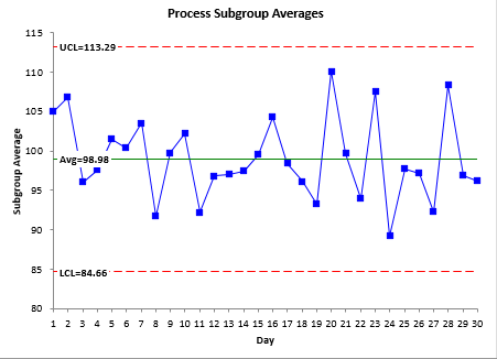
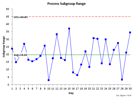
The X-R control chart for these data are shown in Figure 1. The X and the R chart are in statistical control. There are no out of control points. The process is consistent and predictable.
Figure 1: X-R Control Chart for the Process Data

This information can be used to calculate the variation in the individual values you would expect (step 3), i.e., you can determine where essentially all your individual values will lie. The only reason you can do this though is because the process is in statistical control.
Since the process is consistent and predictable, you can move on to step 2. What if the process is not consistent and predictable? How can you calculate the process capability? The answer is simple – you can’t. Yes, you can go through the motions of calculating a Cpk value. It might satisfy the customer or your leadership – but the value you get has no meaning. The data used are not consistent and predictable. You cannot predict where those individual values will lie in the future.
Step 2: Construct a Histogram and Compare to Specifications

Note that when looking at whether the process was in statistical control, we did not say a word about specifications. That is because specifications do not enter into the discussion of whether or not a process is in statistical control. The process itself (and the way you sample it) define the control limits and whether it is in statistical control.
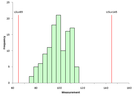
Specifications are set externally to the process – e.g., by the customer. Suppose the specifications for your process are 65 to 145. Using that information and the data from Table 1, the histogram in Figure 2 can be constructed.
Figure 2: Process Data Histogram
The histogram fits easily with the specification limits. Since the process is consistent and predictable, you would expect this to continue. Thus, it appears that your process is meeting specifications fairly easily.
Note that nothing has been said here about whether the data are normally distributed, needs to be transformed or fitted to a non-normal distribution. There is no need to that with this approach. If you have any points that are out of specification, you can easily determine the % out of specification by counting the number of out of specification points and dividing by the total number of points. The distribution issue comes into effect if you are calculating theoretical % out of specification.
In reality, the control chart and the histogram with specifications are all you need to show that your process is capable. The process is in statistical control. Nothing is anywhere near the specification limits. But, people still like to have the Cpk value. So, we will move on to step 3.
Step 3: Determine the Natural Variation of the Process

whereR is the average range and d2 is a control chart constant that depends on subgroup size. The subgroup size for your process is 4. This corresponds to a d2 value of 2.059. The natural variation in the process is then:
The individual values range from 70.36 to 127.6. You would expect essentially all the data to fall within this range as long as the process stays in statistical control. Note that R divided by d2 is the estimate of the standard deviation of the individual values. So,s = 9.54.
Again, note that there is nothing about assuming there is a normal distribution. The fact is, that for just about any set of data, the vast majority of the data falls within +/- 3s of the average.
Step 4: Calculate Cp and Cpk

Cp= ET /NT= (USL-LSL)/6σ =(145-65)/(6(9.54))=1.40
Since Cp is greater than 1, the process is capable of meeting specifications. Another way to look at this number is that it defines how much “elbow room” (as Dr. Wheeler calls it) that your process has. Based on Cp, the process has about 40% elbow room. This means that the specification range is 40% larger than the natural process variation if the process is centered. This process is not centered so you will lose some of that elbow room when looking at individual specifications. This is shown through the Cpk calculation.
The Cpk calculations are given below.
Cpk = Minimum (Cpu, Cpl)
Cpk in this case is 1.19. So, there is about 19% elbow room when you look at the lower specification. Since Cpk is greater than 1, the process is capable of meeting specifications.
Step 5: Combine All the Information When Summarizing Process Capability

- The control chart shows that the process is consistent and predictable
- The histogram shows that the process variation fits easily within the specification range
- The value of Cp and Cpk confirm what the histogram shows
- This process is more than just consistent and predictable – it is capable of meeting specifications – just want you want!
This paints a true picture of the process capability – much more than a Cpk value by itself. You have confidence in this process – and so should your customer and leadership.
Summary
Just looking at a Cpk value does not tell the entire story. The first step – and the most important – is to demonstrate that the process is in statistical control. There is only way to do that and that is through the use of control charts – over an extended period of time. If the process is not in statistical control, you need to work on that and not worry about the process capability. Only when your process is consistent and predictable can you move to the next steps.
The next step is to demonstrate that the process variation fits within the specifications by constructing a histogram with the specifications. Finally, you are ready to calculate the process variation, Cp and Cpk. And the last step is to put it all together to fully describe the process capability.


Very good article. Why are the natural process limits of your Step 1 control chart different than those of your step3 calculation?
The Xbar chart control limits are based on +/- three standard deviations of the subgroup averages. The standard deviation of subgroup averages is equal to the standard deviation of the individual values divided by the square root of the subgroup size (4 in this example). So, the subgroup averages always have less variation thatn the natural limits – in this cae, by a factor of 2.
Cp & Cpk are two terms which are used in day to day life of any manufacutring plant. We use it daily and believe me the ocnfusions are always there, nobody is fully sure of what exactly it is and how to use it in real terms. Your article have clreaed many of my doubts and i am sure it will help our plant performance as well.Thanks again for the wonderful article.
The details about steps to be followed for Process capability were very valuable to me.It provided fantastic information.Thanks for the update and look forward for more.BR
Glad that I found this wonderful website. If I have a set of data where the subgroup size is different, how should I determine which d2 value to be used for the Cpk calculation? If I perform a Ppk calculation, is the Ppk value going to be affected by the difference in subgroup size? Thanks.
The value of Ppk is not affected by the difference in subgroup sizes. It is based on the calculated sigma value which simple takes all the data in one group. For Cpk with varying subgroup sizes, you cannot use one value of d2. You have to determine sigma using a formula. That formula is given here. Of course, the easiest way to do is to purchase SPC for Excel. It does that for you automatically. ?
Bill
Thank you so much. Your articles are great!
Good Read. All aspects are reflective of proper identification of Statistical Control in a process. I do differ on 1 belief however, and that is that Normality of your data is not a requirement to efficiently understand the capability of the process.1. In step one you Created a control chart to identify process stability: Process stability (special causes) are identified based on the distribution of the process. A skewed distribution analyze as a normal distribution would create false flags of special events causing you to fail your first step.2. If by chance the non-normal process passes through the original stability screen. In step 2 it is stated that the calculation for process yield can be completed using Failed Parts/Total Parts. This is TRUE for actual yield but your article is based on Cp and CPK which is not actual yield it is expected yield with the assumption of no shifts or drifts. The yield statement can not apply to a NON-normal distribution because you are using Normal approximations to predict future yield.3. In step 3 for Cp/Cpk you mention that a distribution estimate is 3 standard deviations from the mean (Cpk: to the nearest limit). This is also TRUE, but only applys when the distributions are spread evenly across the mean. If you have a Non-normal population the +3s calculation from the mean does not reflect distribution probability. Thus the Cp/Cpk which are population ESTIMATES can not be considered accurate reflection either.All in All great Article. I believe Normality should be added as your first step. Please provide feedback.
Thanks for your comment. There is a not a requirement for data to be normally distributed to be used in a control chart. Control charts are empirically based – not based on the assumption of data following a normal distribution. Dr. Wheeler has addressed this in detail in a number of his books. It is true that Cpk is based on the assumption of the data being normally distributed. See this link for a discussion of individual charts and non-normal data,
First of all thank you very much for the informative article, it is clear, concise, and not overly cluttered with statistical terminology. I have been doing a lot of reading into Cpk and Ppk recently as we begin to qualify our process for volume production. I have seen in many instances a mention of confidence intervals on Cpk based upon the sample size. To take the data used in the example the sample size is 120 and the calculated Cpk is 1.19. Then I can say with 95% confidence that the Cpk value is actually between 1.03 and 1.35. My question is, why add a confidence interval to Cpk if you have already proved that the process is in control? Is it conventional to target a Cpk of 1.33 or greater even though there is a chance at some confidence level that value could fall below 1.0 based upon the sample size used? I'd love to hear your insight into confidence intervals on Cpk and when to apply them. Thanks!
Thanks for the comments on the article. I am not a fan of confidence intervals on Cpk. Simply complicating things unnecessarily. Once your process is in statistical control and you have enough data in the control chart, there is no need to recalculate control limits, Cpk or anything. Enough data means two things to me: sufficient individual dad ta points (100 is a good number) and sufficient time that the vast majority of sources of variation have had an opportunity to occur. There is always variation, so you will always have a different result if you take another 100 data points. But if your process is in control, those differences are not statistically significant – and probably not significant for your process either. Most important to me is using your knowledge of the process and the key question is has there been enough time for most of the sources of variation to occur in my process.
Hi Bill, again a very nice article.I just wanted your view on the choice of using an XbarR as opposed to calculating the the mean and range and then plotting a Xm chart for both. The XbarR will normally give you more tightnened control limits and thus there is a great chance that the process is showing points outside the the control limits. The Xm chart is more forgiving in this repect and thus the process will be in control but may lead to a lower Cpk as the control limits will be wider (more forgiving). I raise this point as I was a heavy XbarR user until I read an chapter from Wheelers book "Making sense of data" 2003, section 16.1. It details that Shewhart predominantly used XbarR charts but this was because he was looking mostly at manufactruing issues where they were "collecting multiple measurements within a short period of time". Therefore is it correct to use a XbarR chart when you look at 4 values per day, even if it is for 15 days?RegardsIan
Hello Ian,
You are correct that the control limits are tighter for an Xbar-R control chart than for the individauls control chart. However, the Cpk value will essentially be the same whether you group the data or use individuals value assuiming hte proces is stable. The variation in the indiviual values (the standard deviation) will be the same.
You say you get 4 values a day, but only every 15 days? I would probably go with the Xbar-R chart. With indiviuals chart it is best to have somewhat of a constant time frame between points.
The readings that were provided was 4 readings every day for 15 days. Given the comment that Wheeler made that XbarR charts be used for situations as per monitoring manufacturing processes (ie rapid sampling frequencies taken over short time periods, and taken under essentially the same conditions), I was wondering if the XbarR in this case was appropriate as 4 samples each day had the potential to be operating under “different’ conditions. I guess it’s the thing about the data context and rationale sub grouping. But if you do not know is the XbarR dangerous as it has the potential to identify “strong signals” points outside the control limitsI think the problem with with Cp/Cpk and Pp/Ppk is that people quote these without looking at control charts first. I have seen people quoting these indices based upon 3 points, the low number is not obvious as the indices are presented in dashboards and the number of batches is conveniently missed. That’s why I liked the confidence intervals, but I take on board your point mentioned in a previous thread above
You can definitely us e the Xbar-R chart for 4 readings every day for 15 days. The range chart is the within day variation and the Xbar chart is the between day variation. If it is widely out of control, then the variation between days is much larger than the variation within days. This maybe natural – in that case use the Xbar-mR-R within/between charts.
You should always use control charts to ensure that the process is stable – otherwise Cpk and Ppk have no meaning – not to mention those two values will be close if the process is in control.
You need enough degrees of freedom so the estimate the variation is valid. 3 points is ridiculously low – but that is someone wanting to fill in a dashboard and not taking time to learn what those value mean – if anything. For degrees of freedom, please see this link:
https://www.spcforexcel.com/knowledge/control-chart-basics/how-much-data-do-i-need-calculate-control-limits
In step 1, graph no.1 – process subgroup average. How did you calculate UCL:113.29 & LCL:84.66 ??
Please see this article: https://www.spcforexcel.com/knowledge/variable-control-charts/xbar-r-charts-part-1