July 2006
In this issue:
- Statistical Management
- Two Types of Mistakes
- Statistical Signals and Control Charts
- The Funnel Experiment
- Rule 1
- Rule 2
- Rule 3
- Rule 4
- Examples of the Rules
- Video: The Funnel Experiment
- Quick Links
Greetings,
I worked for a chemical company at one time. Part of the process involved the drying of PVC resin in a rotary dryer. The target for the moisture content of the resin was 0.2%. A sample was taken every two hours from the dryer outlet. If the moisture content was over 0.2%, the operator would turn the temperature up to take out more of the water content. If the moisture content was less than 0.2%, the operator would turn the temperature down.
Neither the operator nor management understood the information contained in variation. As a result, the operator was over-controlling the process and actually increasing variation. This e- zine reviews the importance of understanding variation and presents the funnel experiment, a great way of demonstrating the dangers of over-controlling a process.
Statistical Management
To understand variation, it is essential to understand the difference between a process that is in statistical control (stable) and a process that is out of control (unstable). To determine the difference, we must know how to plot points and then decide by some rational method if the process is in control. There are many things we can plot, including weekly sales figures, customer complaints, product responses, inventory, absenteeism, accidents, accounts receivable, turnover, etc.
A key to understanding variation is to plot the points in the order they were produced. For example, you might plot accounts receivable on a weekly basis. After plotting a sufficient number of points, the next step is to question whether the process that produced the data is in statistical control. Why do we want to consider statistical control? The major reason is that the type of action required to improve a process is different for a process that is in control than for a process that is out of control. A major fault, which exists in many places today, is the assumption that every event (defect, mistake, accident) is attributable to someone or is related to one event. For example, suppose this month’s expenditures versus budget (the variance) is slightly higher than last month’s variance. Why did this occur? Is it attributable to one person or one event? We often spend a lot of time looking for these types of answers. The fact is, however, that most troubles with service and production lie in the system and are not attributable to one person or one event.
There are two types of variation. Common cause variation is variation due to the system. Reducing common cause variation is the responsibility of management. Dr. Deming has estimated that 94% of problems are due to common cause variation, i.e., due to faults in the system. Special cause variation is variation due to sporadic, unnatural events. Special cause variation is the responsibility of the front-line personnel to correct. Dr. Deming has estimated that 6% of problems are due to special cause variation.
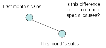
The problem now becomes how to determine if results are due to common cause variation or special cause variation. Is the fact that current sales are less than last month due to common cause variation or special cause variation? Confusion between common and special causes leads to frustration, greater variability and higher costs.
Good management of people and of processes requires the knowledge of how to separate the two kinds of causes. The only good way to do this is through the use of control charts.
Two Types of Mistakes
There are two types of mistakes we can make when looking at data. One mistake is to assume that a data point is due to a special cause when in fact it is due to common cause (mistake 1). For example, we could make this mistake if we looked at each month’s sales figures and tried to find one reason why sales were up or down. The second type of mistake is to assume that a data point is due to common cause when in fact it is due to special causes (mistake 2). For example, we could make this mistake by never looking at reasons for changes in sales figures, assuming that the changes are always due to the normal variation in the sales process.
There is no hope to avoid both these mistakes all the time. In other words, we will make the first mistake sometimes and the second mistake sometimes. Thus, management is about making mistakes. What we need are some rules to help us minimize the loss due to these mistakes. These rules are the control limits on control charts.
Statistical Signals and Control Charts
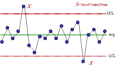
Assume that a process is in statistical control (only common cause variation present). If you plot 1000 points from this process, only three will be beyond the control limits. Therefore, anytime a point is beyond the control limits, there is only a 3 in 1000 chance that it is due to common causes. Since this probability is low, it probably is due to a special cause. Thus, the control limits help minimize how often we make mistake 1. (Note: since no process is really unwavering, you cannot assign any probability that a statistical signal may be wrong.)
We will make mistake 2 more often than mistake 1. Points that lie between the control limits are assumed to be due to common cause variation. It is possible that a special cause is present from time to time but the point will still lie between the control limits. We are willing to make this mistake more often because it does not require any action from us. If a point is out of control, it takes time and energy to find out what happened. We want to be sure that there is a special cause present before we start looking for it. Control limits help us accomplish this.
Control charts help us determine the type of variation present. This is important to know because the strategies for improving a process that is in statistical control is different from the strategies for improving a process that is out of statistical control.
If a process is out of control, the discovery and removal of special causes is usually the responsibility of the front-line personnel (those closest to the process). However, some can be removed only by management. It is important to remember that removing special causes from a process is not improving the process. You are merely putting the process where it should be.
A process is in statistical control if there are no special causes present. It represents a random process that is predictable in the near future. For example, we don’t know what the exact value of the next data point will be, but we do know that it will fall between the control limits. We also know what the long term average of the process will be. No action is taken on the “ups” and “downs” in the process. Being in statistical control is not a natural state. It is obtained by eliminating special causes one by one. In addition, costs are predictable and at a minimum for a process that is in control. Productivity is at a maximum.
The responsibility for improving a process in statistical control lies with management. Front-line personnel may have excellent suggestions on how to do this. Improving a process that is in control may mean changing the average or reducing variation. It is a never-ending process. The system must be changed to improve the process. Examples of system changes include new machines, new methods, and new materials.
What happens if you use the wrong strategy for improving a process? For example, suppose your process is in control. One point comes in below the average. You decide to adjust the process to compensate for this and you continue to adjust the process any time a point is below average. What have you done to the process? In reality, you have increased the variation in the process. It is possible that you have created a process that is now out of control.
Suppose your process is out of control and you try to improve the process by changing the system. For example, suppose you want to decrease the average turnaround time for memos. To accomplish this, you buy a new software package. The next point you get is below the average. Have you improved the process? You don’t know, because the original process was not in control.
The first step in continuous quality improvement is to remove the special causes of variation. Only then can true process improvement begin through the reduction of common causes of variation. The next section highlights what can happen if you ignore the information contained in variation.
The Funnel Experiment
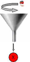
An excellent example of over-controlling is the funnel experiment described by Dr. Deming. The objective of the funnel experiment is to drop a marble through a funnel and hit a target.A point on a level surface is designated as the target. A funnel is held a certain distance above the surface. A marble is dropped through the funnel. The spot the marble comes to rest on the surface is marked. This is repeated for at least 50 drops for each of four different rules.Each of the four rules is discussed below.
- Rule 1: Leave the funnel fixed over the target.
- Rule 2: For every drop, the marble will come to rest a distance “z” from the target. Rule 2 is to move the funnel a distance -z from its last position.
- Rule 3: Move the funnel a distance -z from the target after each drop of the marble that ends up a distance z from the target. Note that Rule 2 moves the funnel based on the funnel’s last position. Rule 3 moves the funnel a distance from the target.
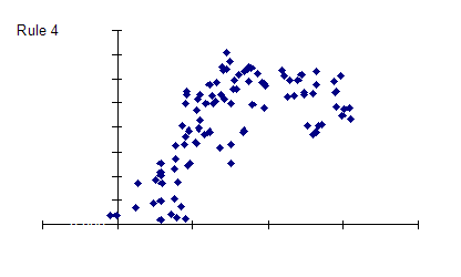
- Rule 4: Rule 4 is simply to set the funnel over where the last drop came to rest.
Rule 1
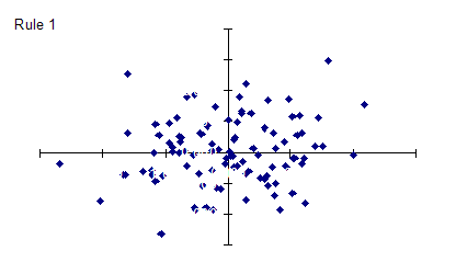
Rule 1 is to leave the funnel fixed over the target. The marble is dropped at least 50 times and the spot where the marble comes to rest is marked each time. The resulting pattern is shown in the adjoining figure. This is a computer simulation of 100 marble drops. The target is where the solid lines cross.
As can be seen in the figure, the variation is a rough circle and is stable. Surely we can do better than this! This circle is too big. Why don’t we simply adjust the funnel after each drop so the next drop will be closer to the target?
Rule 2
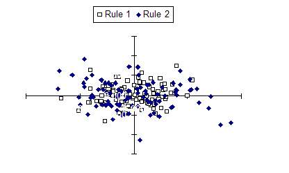
As can be seen in this figure, the pattern for Rule 2 is also circular and stable. However, the circle is larger than for Rule 1. It is about 41% larger. Using Rule 2 actually increases the variance of the process by a factor of 2 over Rule 1.
Rule 2 is often used in business by people just trying to do their best. This is why it is important to understand the information in variation. By responding to variation that is common cause as if it were special cause, you are increasing the variation in your process.
Rule 3
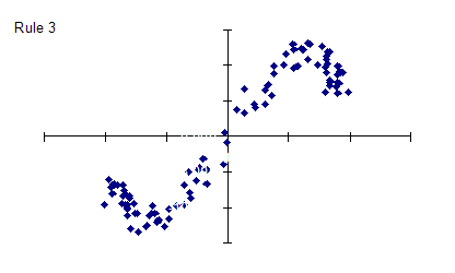
Under Rule 3, the marble drop swings back and forth. The pattern looks similar to a bow tie. This is not a stable process. The amplitude of the swings will continue to increase.
Rule 4
Examples of the Rules
Examples of Rule 2 include:
- Feedback mechanisms that respond to a single data point
- Adjusting a process when a part is out of specifications
- Operator adjustments without the aid of control charts
- Changing company policy based on the latest attitude survey
- Recalibrating instruments to a standard
- Adjusting the quota to reflect current output
- Using variances to set budgets
- Stock market reaction to last month’s deficit
Examples of Rule 3 include:
- Illicit drugs. Enforcement improves so drugs become scarcer. The price goes up which stimulates the import of more drugs. The cycle repeats.
- Gambler increases his bet to cover losses
Examples of Rule 4 include:
- History passed down from generation to generation.
- Worker training replacements in succession.
- Adjustment of time of meeting based on last actual starting time.
- Use of last board cut as a pattern for the next board.
- Sitting in a circle with a number of people. One person whispers a secret to the next person who in turns whispers it to the next person and so on.
Note: Permission to use the Media Gallery photo of Dr. Deming granted by Diana Deming Cahill of the W. Edwards Deming Institute.
Video: The Funnel Experiment
