October 2026
 What is the Cpk value of your process? Odds are that you know it. You probably have customers who want to know it – and maybe require it be above some value like 1.33. You may get questions about the other process capability indices (Cp, Pp, Ppk) as well. But you probably don’t get this question very often:
How close is your process running to target?
The four process capability indices will not answer that question for you. Your process can have a wonderful Cpk value and still be running well away from target – the target where you and your customer want it to be.
Enter Cpm. Cpm is a process capability index that takes the target into account. This publication looks at what Cpm is, how it is calculated, and how to interpret it.
In this issue:
- Cp, Cpk and the Missing Target
- Taguchi’s Loss Function
- Defining Cpm
- Cpm When the Target is Not the Midpoint
- Cpm with Only One Specification Limit
- Example: Calculating Cpm
- Interpreting Cpm
- Summary
- Quick Links
Please feel free to leave a comment at the end of the publication. You may download a pdf copy of this publication at this link.
Cp, Cpk and the Missing Target
Let’s start with a quick review of the process capability indices most of us use. Cp is the capability ratio. It compares the width of the specifications to the natural variation in the process:
Cp = (USL − LSL) / 6σ
where USL is the upper specification limit, LSL is the lower specification limit, and σ is the process standard deviation estimated from within-subgroup variation (for example, the average moving range divided by 1.128 for individuals data). Cp says nothing about where the process is located – or what the target value is. It only tells you whether the process could fit within the specifications if it were centered. Figure 1 demonstrates this for Cp.
Figure 1: Cp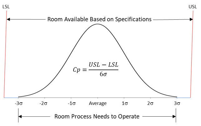
Cpk adds the location. It is the minimum of Cpu and Cpl:
Cpu = (USL − X) / 3σ
Cpl = (X − LSL) / 3σ
Cpk = Minimum(Cpu, Cpl)
where is the process average. Figure 2 shows Cpk. Cpk is based on the specification limit that is closest to the average. In the figure below, that is the lower specification limit.
Figure 2: Cpk

Pp and Ppk use the same equations but with s, the standard deviation calculated from all the data, in place of σ. You can read more about these four indices in our SPC Knowledge Base article What Do the Process Capability/Performance Metrics Measure?
What is missing from all these equations? The target. Cpk measures how far the average is from the nearest specification limit. But it doesn’t account for the target – or care where the target is. Consider two processes, both with specifications of 90 to 110 and a target of 100.
Process A has an average of 100 and a standard deviation of 3.33. Process B has an average of 106 and a standard deviation of 1.33. These two processes are shown in Figure 3.
Figure 3: Two Processes with the Same Cpk
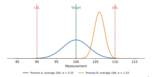
Process A is centered on the target. Process B has much less variation but is running 6 units above the target. The processes are definitely different. What is Cpk for each process?
Cpk for Process A:
Min( (USL −X ) / 3σ, (X − LSL) / 3σ)=Min[(110 − 100)/3(3.33), (100 − 90)/3(3.33)] = 1.0
Cpk for Process B:
Min( (USL − X) / 3σ, (X − LSL) / 3σ)=Min[(110 − 106)/3(1.33), (106 − 90)/3(1.33)] = 1.0
The Cpk values are the same. Does this mean that both processes are the same? No, it is clear from Figure 3 that the processes are different. If your customer wants a process centered at 100 and you are delivering a process centered at 106, how do you think the customer will like that? It is not what they want.
Cpk cannot tell the difference between these two processes. Cpm can.
Taguchi’s Loss Function
One definition of quality is being on target with minimum variation. But most companies don’t follow that definition. Instead, they focus on whether a part is within specification or not. If a part is within spec, you are happy. The assumption is there is no loss as long as the part is within specification. 109 is the same as 100.
Genichi Taguchi, a quality guru, did not see it that way. He argued that any departure from the target results in some loss – to the customer, to the next process, or to society. The farther you are from the target, the greater the loss. He modeled this loss as a quadratic function:
L = k(x − T)²
where L is the loss, x is the measured value, T is the target, and k is a constant that converts the deviation into a cost. Figure 4 shows the loss function.
Figure 4: Taguchi’s Loss Function
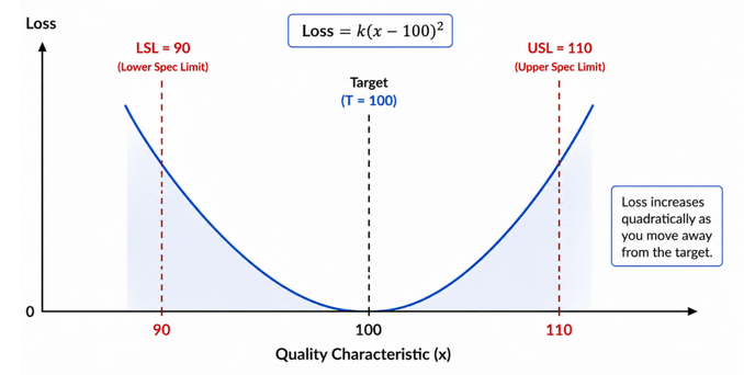
If you average the loss over all the product made, the average loss is proportional to the average squared deviation from the target. That average squared deviation has two pieces – the variation around the process average plus the squared distance between the average and the target:
E[L] = k[(μ – T)² + σ²]
where E[L] = expected loss for the process, k = the loss constant, μ = the process average, T = the target, and σ² = the process variance. So, there are two ways to lose: having too much variation and being off target. Cpm is built on this idea.
For more information on this, please see our SPC Knowledge Base article Taguchi’s Loss Function.
Defining Cpm
T. C. Hsiang and Taguchi described Cpm in 1985. It was formalized as a capability index by Chan, Cheng and Spiring in 1988 (“A New Measure of Process Capability: Cpm.” Journal of Quality Technology, 20(3), 162–175).
When the target is the midpoint of the specifications, Cpm is defined as:
Cpm = (USL − LSL) / 6τ
This looks just like Cp. The difference is the denominator. Cp uses σ, the variation around the process average. Cpm uses τ (tau), the variation around the target. If the process is centered right on the target, τ is essentially the same as the standard deviation. As the process average moves away from the target, τ gets larger and Cpm gets smaller – even if the variation in the process does not change at all.
So, what is tau? Tau is the root mean square deviation of the data from the target. It is calculated just like a standard deviation, except that each value is compared to the target instead of the average:
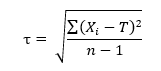
where Xᵢ is each individual value, T is the target, and n is the total number of values. Note that n − 1 is used in the denominator, the same as when calculating the sample standard deviation, s. If your data are in subgroups, all the individual values are used; τ is based on all the data, not on within-subgroup variation.
There is a useful relationship between τ, the standard deviation (s) and the average. The sum of squared deviations from the target can be split into two pieces:
Σ(Xᵢ − T)² = Σ(Xᵢ − X)² + n(X − T)²
The first piece is the variation around the average. The second piece is how far the average is from the target. Dividing by n − 1 gives:
τ² = s² + [n/(n − 1)](X − T)²
This is Taguchi’s average loss in another form. For any reasonable sample size, n/(n − 1) is close to 1, so τ² is essentially:
τ² = s² + (X − T)².
Since τ is based on all the data, Cpm is really more like the process performance indices (Pp, Ppk) than the process capability indices (Cp, Cpk). As always, the results only have meaning for predicting the future if the process is in statistical control.
Let’s go back to Processes A and B, which had the same Cpk value but were centered at two different spots. We will use the equation above to determine τ. For Process A, the average is on target so X − T = 0 and τ = s.
Cpm = (USL − LSL)/6(τ) = 20/6(3.33) = 1.
For Process B, the average is 6 above the target, so X − T = 6. τ is then the square root of 1.332 + 62 = 6.15. Cpm is then 20/6(6.15) = 0.54. This is very different than the Cpm for Process A. Process B pays a big penalty for running off target.
The target is not always the midpoint of the specifications. What happens then? Let’s see.
Cpm When the Target is Not the Midpoint
The target is not always the middle of the specifications. For example, a fill weight may have specifications of 490 to 520 grams with a target of 500 grams. In this case, the target is closer to the LSL than the USL. Using (USL − LSL)/6τ would overstate the capability because it treats the distance from the target to the two limits as being the same.
When the target is not the midpoint, Cpm uses the shorter distance from the target to a specification limit:
Cpm = Minimum(USL − T, T − LSL) / 3τ
This is the general form of Cpm with two specification limits. When the target is the midpoint, USL − T and T − LSL are both equal to half the specification width, and the equation reduces to (USL − LSL)/6τ. So, you can always use this form.
Cpm with Only One Specification Limit
Cpm can also be calculated when there is only one specification limit, as long as there is a target. With only an upper specification limit:
Cpm = (USL − T) / 3τ
With only a lower specification limit:
Cpm = (T − LSL) / 3τ
These are similar to Ppu and Ppl, with the target taking the place of the average and τ taking the place of s.
Example: Calculating Cpm
Let’s work through an example. Table 1 contains 25 individual results from a process. The specifications are 90 to 110 and the target is 100.
Table 1: Process Data
| Sample | Value | Sample | Value | |
| 1 | 104.2 | 14 | 102.7 | |
| 2 | 104.7 | 15 | 104.2 | |
| 3 | 103.8 | 16 | 105.3 | |
| 4 | 102.8 | 17 | 102 | |
| 5 | 103.5 | 18 | 103.5 | |
| 6 | 102.6 | 19 | 101.2 | |
| 7 | 104.3 | 20 | 102.1 | |
| 8 | 106.3 | 21 | 101.3 | |
| 9 | 103.4 | 22 | 103.8 | |
| 10 | 103.2 | 23 | 102.2 | |
| 11 | 105 | 24 | 104.6 | |
| 12 | 104.8 | 25 | 104.5 | |
| 13 | 104.4 |
We will leave it to you to produce the individuals control chart for this data. It is in statistical control, so we can continue with calculating the capability. A histogram of the data is shown in Figure 5. It includes the specifications and target.
Figure 5: Histogram of Process Data
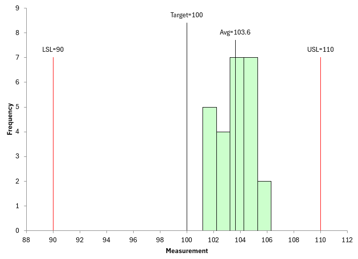
The points lie easily within the specifications, so if you believe “in spec is good,” you are happy. But the average is well above the target – not what the customer wants.
The basic statistics are:
- n = 25
- = 103.616
- s = 1.275
- Average moving range = 1.371, so σ = 1.371/1.128 = 1.215
Step 1: Calculate the squared deviation of each value from the target.
For the first value, (104.2 − 100)² = 17.64. Do this for all 25 values and add them up:
Σ(Xᵢ − 100)² = 365.90
Step 2: Calculate τ.
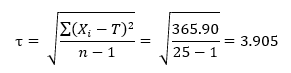
Step 3: Calculate Cpm. The target is the midpoint, so:
Cpm = Minimum(110 − 100, 100 − 90) / 3(3.905) = 10 / 11.715 = 0.85
Figure 6 shows a process capability analysis for this data.
Figure 6: Capability Analysis
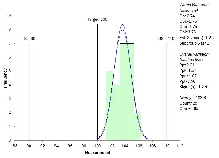
This analysis, like the histogram above, was done using the SPC for Excel software. Figure 6 shows the other capability indices. How does Cpm compare to the other indices?
The results are summarized in Table 2.
Table 2: Capability Results (Specifications 90 to 110, Target 100)
| Index | Value |
| Cp | 2.74 |
| Cpk | 1.75 |
| Pp | 2.61 |
| Ppk | 1.67 |
| Cpm | 0.85 |
Cpk of 1.75 and Ppk of 1.67 look very good. Cpm of 0.85 does not. Why the difference? Let’s split the 365.90 into its two pieces:
Σ(Xᵢ − X)² = 39.01
n(X − T)² = 25(103.616 − 100)² = 326.89
Only 39.01 of the 365.90 (about 11%) comes from variation around the average. The other 89% comes from the process running off target. The process has very little variation; it is simply aimed at the wrong place. The good news is that this is often the easiest problem to fix. Moving the process average to the target would raise Cpm to about the same value as Pp.
Interpreting Cpm
Cpm is interpreted like the other indices: the larger, the better. A Cpm of 1 means that 3τ just fits between the target and the closest specification limit. But the real value of Cpm comes from comparing it to the other indices (these comparisons assume the target is the midpoint of the specifications; with an off-center target, Cpm will be lower than Pp even when the process is exactly on target):
- If Cpm is close to Pp (or Ppk with one specification), the process is running close to the target.
- If Cpm is much smaller than Pp, the process is off target. The problem is aim, not variation.
- If Pp is small and Cpm is small, the process has too much variation, regardless of where it is aimed.
Cpm is especially useful when it matters where the product falls within the specifications – for example, when two parts must fit together. Two mating parts can each have a high Cpk and still fit poorly if one runs high and the other runs low. Cpm will flag that problem; Cpk will not.
And remember: Cpm, like all capability indices, is only meaningful if the process is in statistical control. If the process is not stable, you cannot predict what it will do in the future, and no capability index will help you.
Summary
This publication looked at Cpm. Cp, Cpk, Pp and Ppk all ignore the target. Two processes can have the same Cpk and be in very different places relative to where the customer wants them.
Cpm replaces the standard deviation with τ, the root mean square deviation from the target, so that being off target is penalized just like excess variation.
With two specification limits, Cpm is the shorter distance from the target to a specification limit divided by 3τ; this reduces to (USL − LSL)/6τ when the target is the midpoint. With one specification limit, Cpm is the distance from the target to that limit divided by 3τ. Comparing Cpm to Pp quickly tells you whether your problem is too much variation or a process that is simply not aimed at the target.