
August 2026
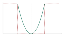 Back in the early 1980’s, I worked in a manufacturing plant as Chief Chemist. I was just starting to learn about statistical process control. The plant I worked at had a simple approach to quality: specifications. If the product was within specifications, it was good and could be shipped. If the product was outside specifications, it was bad and had to be reworked or scrapped. But only after testing it again to be sure it was out of specifications. If this re-sample was good, the previous sample was a lab error. The product now magically was good – it was in specifications. Simple!
Then along came Dr. Taguchi. He challenged this way of thinking about quality. He believed there wasn’t anything magical about a specification limit – a point where a product suddenly goes from good to bad. This publication examines Dr. Taguchi’s approach that quality is on target with minimum variation about that target. It is built around his loss function.
In this publication:
- Specification Approach to Quality
- Genichi Taguchi
- The Taguchi Loss Function
- Average Loss for a Process
- The Reality of the Loss Function
- Control Charts and the Loss Function
- Summary
- Quick Links
Please feel free to leave a comment at the end of this publication. You can download a pdf copy of this publication at this link.
Specification Approach to Quality
This approach to quality is simple:
- Within specifications: product is good
- Outside specifications: product is bad
This is depicted in Figure 1 for a process with a target of 100 and specifications from 90 to 110.
Figure 1: Specification Approach to Quality
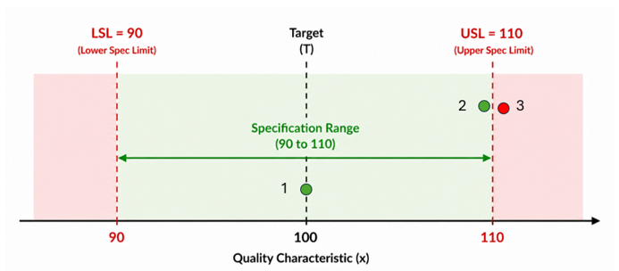
Sample 1 in the figure is right on target. So, the product is good. Life is great. The next sample, 2, is 109.9. Again, the sample is within specifications. Life is still good. Sample 3 is 110.1. This sample is out of specifications. The product is not good. Question: do you really believe that there is significant difference between samples 2 and 3? Is 109.9 significantly different than 110.1? Maybe but most likely not in this scenario. But we call sample 2 “good” and sample 3 “bad”.
This was really the definition of quality presented by Philip Crosby:
Quality is conformance to requirements
Requirements are the specifications. Of course, specifications were around long before Crosby. He just formalized it. Last month’s SPC Knowledge Base publication was “What is Quality? Definitions from the Quality Gurus of the 20th Century.” See this publication for more information on Crosby as well as six other gurus including Dr. Taguchi.
Enter Dr. Genichi Taguchi. Dr. Taguchi said conformance to specifications was wrong. Let’s see what Dr. Taguchi said to do.
Dr. Genichi Taguchi
Dr. Taguchi defined quality as the following:
Quality is the minimum loss imparted to society from the time a product is shipped.
How do you accomplish this minimum loss? By meeting the following three items:
- A product should hit its target value, not merely stay within specification limits.
- Variation around the target should be minimized.
- Any deviation from the target causes a loss to society, even if the product remains within specifications.
So, in his view, any deviation from target, no matter how small, creates a loss for the customer, the company, and society. And, in his view, the further you are from the target the more the loss grows. Dr. Taguchi focused on the target and on reducing variation about that target. This is a very different view of quality – and it leads up to what is now one of the most important concepts in quality:
On target with minimum variation
What happens when a product doesn’t perform as intended? Lots can happen including warranty costs, product returns, extra service calls, downtime, etc. All this can create an unhappy customer.
Dr. Taguchi believed this loss started with any deviation from target. On target, you are minimum loss. As you move away from the target the loss increases. If you move even further away, the loss can increase significantly.
The Taguchi Loss Function
Dr. Taguchi developed a loss function to describe mathematically what happens when there is a deviation from target. The loss function is shown in Figure 2.
Figure 2: Taguchi Loss Function
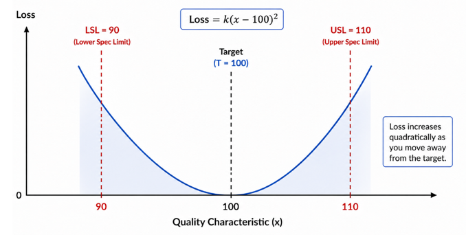
For a characteristic where there is a specific target value, the Taguchi loss function is written as:
L(x) = k(x – T)²
where: L(x) = the loss associated with a particular value of the quality characteristic, x = the actual value of the quality characteristic, T = the target value (T = 100 in the example) and k = a constant that converts the deviation from target into a monetary loss
Let’s examine this simple equation. Suppose your sample result (x) is 100, right on target. The loss is then:
L(x) = k(x – T)2 = k(100-100)2= 0
Now suppose your x result is 105, for a deviation from target of 5. There is a loss since you are not at target. The loss is then:
L(x) = k(x – T)2 = k(105-100)2 = k(5)2 = 25k
Note that the deviation from target (5 in this example) is squared. So, the loss is 25, not 5. The square term causes the loss to increase more rapidly the further away the result is from the target. If the deviation from the target is increased from 5 to 10 (doubles it), the loss becomes 100 (increases by a factor of 4).
To really use the loss function in terms of a financial loss, you estimate a value for k. You can do this if you can estimate the monetary loss associated with reaching a certain deviation from target.
This is often not a simple thing to do. But you can still estimate the loss by just taking the square of the deviation from the target. Just use k = 1 until you have estimated what k is.
Average Loss for a Process
So far, we have looked at the loss for one individual result. But processes produce many individual results. What we really want to know is the average loss generated by the entire process.
For the quadratic Taguchi loss function, the expected loss for a process can be written as:
E[L] = k[(μ – T)² + σ²]
where E[L] = expected loss for the process, k = the loss constant, μ = the process average, T = the target, and σ² = the process variance.
Look at the two terms in the brackets (μ – T)² and σ². The first represents the loss due to the process average being off target. The second represents the loss due to variation. You want to reduce both of those. So, the objective is still clear:
On target with minimum variation
Let’s look at each of these: target and variation. Suppose we have a process making widgets that has no variation. Not possible, but it allows us to look at the impact of being off target. Suppose the process average is 1.03. Let’s say we estimated k to be $1. The loss due to being off target this then:
E[L] = k[(μ – T)² + σ²] = 1*(103 – 100)2 = $9 per unit
If we make 10,000 widgets per year, the estimated loss becomes: 10,000 × $9 = $90,000.
That is a lot of money from being off target by just 3.
Remember a process can be stable – in statistical control and within specifications. But if it is not operating at target, there is a loss.
Now assume our process is right on target so μ – T = 0. The expected loss then becomes:
E[L] = kσ²
Suppose k = $1 and the standard deviation is 2. Then the expected loss is
E[L] = 1*(4) = $4 per widget
For 10,000 widgets, the loss is 10,000*$4 = $40,000. Variation causes losses as well.
The Reality of the Loss Function
The loss function equation makes the concept mathematically precise, but most of the time, the value of k is not estimated. It is very difficult to assign a loss to specific deviation from target, e.g., what is the loss of being at 103 instead of being on target. But the actual loss is not what is important. It is the message that the loss function sends:
Don’t aim simply to be within specifications. Aim to be on target with minimum variation.
Control Charts and the Loss Function
So, the objective is on target with minimum variation. How do we know whether this is happening? This is where control charts come into view. A control chart allows us to see the process behavior over time.
The individuals (X-mR) control chart is widely used today. It is really two charts:
- The X control chart where each individuals value is plotted.
- The mR control chart where the range between consecutive values is plotted.
The figure below is an example of an X-mR chart. The target for the process is 100. The first chart is the X chart. It is shown in Figure 3.
Figure 3: X Chart
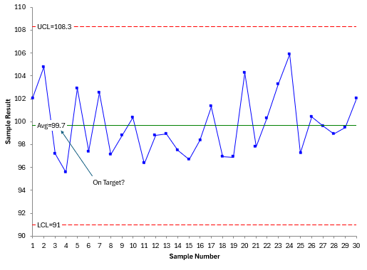
The individual values are plotted on the X chart. After enough points, the process average is calculated along with the upper control limit (UCL) and lower control limit (LCL). A control chart is used to separate common causes of variation from special causes of variation. Common causes of variation are the normal process variation – the noise in the process. If there are no points beyond the control limits or patterns (like 8 in a row below the average), the process just has common causes of variation. It is in statistical control. It is said to be consistent and predictable – a stable process. If there are points beyond the control limits or patterns present, the process has special causes of variation present. It is not consistent and predictable.
On the X chart, there are no points beyond the control limits or patterns. The X chart is said to be in statistical control.
When the X chart is stable, you can ask the question:
Does the process average equal the target?
If it does, the process is on target. In this example, the target is 100. The process average is 99.7. So, is the process on target? It is close and may be close enough to meet your needs.
The second chart is the mR chart. It is shown in Figure 4. It represents the variation in the process. The average moving range is a measure of the variation in the process. So, on target with minimum variation. What is this minimum variation? It is the variation that exists when the process is in statistical control, i.e., the moving range chart is in statistical control.
Figure 4: mR Chart
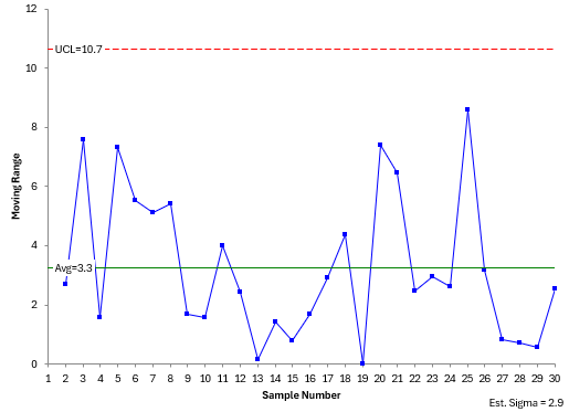
This mR chart is in statistical control, so it is operating at minimum variation. Note this is the minimum variation for the current process. If you there is too much variation even when the process is in control, you will need to reduce the variation. Since the process is in stable, this means you must fundamentally change the process to reduce the variation.
Please see our SPC Knowledge Base for more information on control charts.
Summary
This publication examined Taguchi’s loss function. It was compared to the specification approach. The loss function uses a quadratic function to look at how loss occurs anytime you are not on target. The relationship between the control charts and the loss function was shown.