All Factor Analysis Worksheet Help
Home » SPC for Excel Help » Analysis Help » DOE (Design of Experiments) Help » Two Level Designs: Analysis Help » All Factor Analysis Worksheet Help
The various parts of this worksheet are described below.

Design Table
The design table is at the top of the All Factors Analysis worksheet. This classic design table shows the standard runs and the results. The design table for the etch rate example is shown below. The significant effects are in bold in the row labeled ‘Effects.’
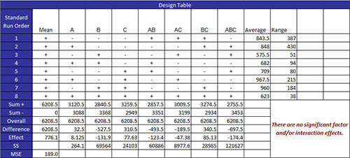
The standard run number is given in Column A, followed by columns for the mean and each factor and interaction in the design. The last two columns are the average and range. The average is the average result for the runs at each standard condition. For example, standard run 1 was run twice during the design (actual runs 9 and 14). The two results were 550 and 604. So, the average is (550+604)/2 = 557. The range is the maximum – minimum for the standard run. For standard run 1, the range is 604 – 550 = 54.
The information below the design table starting with the row labeled “Sum +” is the table analysis using Yates’s algorithm. This will be demonstrated using Factor A results. The rows perform the following functions:
- Sum +: sums the results for a factor at its high level (+);
- Factor A: Sum + = 659.5 +638.5 +808.5 + 794.5 = 2901
- Sum -: sums the results for a factor at its low level (-)
- Factor A: Sum – = 577 + 617 + 1044.5 + 1069 = 3307.5
- Overall: The sum of the sum + and sum – values (this was used as a check on calculations and is the same for all factors)
- Factor A: Overall = (Sum +) + (Sum -) = 2901 + 3307.5 = 6208.5
- Difference: The difference between the sum + and the sum – values; this represents the difference between the sum of the results at the factor’s high level and the sum of the results at the factor’s low level.
- Factor A: Difference = (Sum +) – (Sum -) = 2901 – 3307.5 = -406.5
- Effect: This is the effect of the factor. It is determined by dividing the difference by the number of plus signs in the column. This effect is the difference in the average for the results at the high level of the factor and the average of the results at the low level of the factor. (Note: the effect under the mean column is the average of all the factorial runs.)
- Factor A: Effect = Difference/4 = -406.5/4 = -101.625
- SS: This is the sum of squares for the factor. This the number of replications times the difference squared divided by the total number of factorial runs (N).
- Factor A: SS = (NReps*Difference)^2/N = (2*-406.5)^2/16 = 41,310.56
The last row in this section is labeled MSE. This stands for Minimum Significant Effect. It is one way of determining which effects are significant. The equation for MSE is:
MSE = tσ(SQRT(4/N)
where t is the t value for 95% confidence with the degrees of freedom = number of factorial observations – number of cells,σ is the estimated standard deviation obtained from the range values, and N is the total number of factorial runs. In this example, MSE = 47.7028. If there is only one replication, a different method is used to determine which factors are significant.
This value of MSE is compared to the effects in the design table. Any absolute value of an effect that is greater than MSE is considered significant. The program changes these effects to bold (in the effects row). As can be seen from the design table above, A, C and AC are significant effects.
Range Chart
When multiple replications are run, the program uses the range values to estimate the variability in the process and to check for out of control situations. The output for the range control chart on the All Factors Analysis Worksheet is shown below as well as the calculations.
The average range is calculated along with the upper control limit (UCLr) and the lower control limit (LCLr). The range values are compared to the control limits. If none of the range values are beyond these limits, the ranges are in statistical control. If any range is beyond these limits, there is evidence of a special cause of variation that may make the results suspect.
The average range and the control limits are calculated using the following equations:
R = ΣRi/k
UCLr = D4R
LCLr = D3R
where Ri is the range of standard run i, k is the number of range values, and D4 and D3 are control chart constants that depend on the number of replications (the subgroup size).
There is no lower control limit on a range for 2 replications. The values for D4 and D3 for various subgroup sizes are available in many publications and on our website. Since no range value is above 158.8579, we conclude that the ranges are in statistical control and there were no special causes present when the experimental design was run. The residuals analysis will also check to determine if there were any issues present when the design was run.
Note that the average range is used to estimate the value of the standard deviation used in the MSE equation above (where d2 is a control chart constant that depends on the number of replications):
σ= R/d2
ANOVA Table for Factors and Interactions
The next portion of the All Analysis Factor worksheet is the ANOVA table for the factors and interactions. The output for this example is shown below. The significant effects are those with a p-value ≤ 0.05. A p-value is in red if it is less than 0.05. If the p-value is between 0.05 and 0.20, the p-value is in blue. This effect may or may not be significant. It is border-line and probably should be considered for inclusion in the model. In the example, A, C and AC are significant. This agrees with the result from the design table.
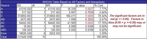
The columns in the ANOVA table are:
Source: the source of variation which includes the factors and interactions in the model as well as the error and the total
SS: sum of squares for each source of variation
The sum of squares for the factors and interactions are given in the design table. The model sum of squares (SSModel) is the sum of the factors’ and interactions’ sum of squares. The total sum of square (SSTotal) is given by the equation below where yi represents an experimental result and N is the total number of experimental runs:
SSTotal = Σyi2 + (Σyi)2/N
The error sum of squares is determined by subtracting the factor and interaction sum of squares from the total sum of squares:
SSError = SSTotal – SSModel
df: degrees of freedom
The degrees of freedom for each factor and interaction is 1 since these are two level designs. The model degrees of freedom (dfModel) is equal to the number of factors and interactions in the model. The total degrees of freedom (dfTotal) is equal to the total number of runs minus 1:
dfTotal= N – 1
The error degrees of freed (dfError) is the given by:
dfError = dfTotal – dfModel
MS: mean square
The mean square for a source is the variance associated with that source and is determined by dividing the source sum of squares by the degrees of freedom for that source:
MS = SS/df
F: value from the F distribution
The F Value for a source of variation is used to compare the variance associated with that source with the error variance. F = MS/MSE where MS is the mean square for a source and MSE the mean square error.
p-Value: the probability value that is associated with the F Value for a source of variation
It represents the probability of getting a given F Value if the source does not have an effect on the response. If the p-value is <=0.05, it is considered to have a significant effect on the response. A p-value above 0.20 is not considered to have an effect on the response. If the p-value is between 0.05 and 0.20, it or may not have a significant effect.
% Cont: the % of the total sum of squares the source of variation accounts for
Smaller p-values will generate larger % contribution. % Cont = SS/SSTotal where SS is the sum of squares for a given source of variation.
ANOVA Table for the Model
The model’s ANOVA table is listed next on the All Factors Analysis worksheet. The output for this example is shown below.
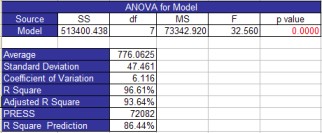
The columns in the ANOVA table have been explained above. There are several pieces of information below the ANOVA table.
Average: the average of the experimental runs
Standard deviation: the square root of the mean square error
Coefficient of variation: the error expressed as a % of the average, 100(Average/Standard Deviation)
R Squared: measures the proportion of the total variability measured explained by the model
Adjusted R Squared: the value of R squared adjusted for the size of the model (the number of factors in the model)
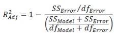
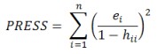
PRESS: Predicted Error Sum of Squares is a measure of how well the model will predict new values and is given below where ei is the ith residual and hii is the diagonal element of the hat matrix (H=X(X’X)-1X’)
R Squared Prediction: indication of the predictive capability of the model; the percent of the variability the model would be expected to explain with new data
Factor Information
Information on the factors is listed next on the All Factors Analysis worksheet. This information includes the factor, degrees of freedom, the standard error and 95% confidence limits. The output for this example is shown to the below.
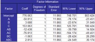
Factor: the intercept, factors and interactions included in the model
Coeff: the regression coefficients for the factors
Degrees of Freedom: the degrees of freedom associated with the factor (always 1 for two level designs)
Standard Error: the estimated variance of the factor which is defined as the following for n = number of replications and k = the number of factors:
95% Upper and Lower Confidence Limits: The upper and lower 95% confidence limit around the coefficient; if it contains zero, the factor is usually not significant
Confidence Limit = b +/- t(0.05, dferror)*se
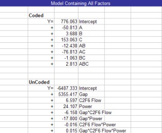
Model Containing All Factors
The last part of the All Factors Analysis worksheet contains the model for all the factors based on the coefficients given above. The coded model is based on the coded levels (-1 to 1) for the factors and interactions. The uncoded model is based on the actual examples. The output for the example is shown below.