Regression Help
Home » SPC for Excel Help » Cause and Effect Help » Regression Help
This page shows how to perform multiple linear regression using SPC for Excel. This page contains the following:

Example
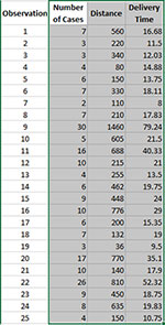
We will use an example from Montgomery’s regression book. An engineer employed by a soft drink beverage bottler is analyzing what impacts delivery times. He decides the two factors that impact the time could be the number of cases a driver delivers, as well as how far the driver has to walk at the customer’s facility. He has collected 25 observations for delivery time (minutes), the number of cases, and distance walked (feet). The data are shown below. We want to use this data to determine if either factor impacts delivery time, and if we can build a model to predict delivery time. The steps below show how to do this using the SPC for Excel software. In this example, we are using the following model:
Y = bo + b1x1 + b2x2
where:
- Y = response variable (delivery time)
- x1 = predictor 1 (number of cases)
- x2 = predictor 2 (distance walked)
- bo = intercept
- b1 = coefficient for predictor 1
- b2 = coefficient for predictor 2
Data Entry
Enter the data into a spreadsheet as shown below. The data can be downloaded here. The data must be in columns with the variable names in the first cell of the column.
Running the Regression
- 1. Select the shaded area (including the headings). You can use “Select Cells” in the “Utilities” panel of the SPC for Excel ribbon to quickly select the cells.
- 2. Select “Regression” from the “Cause and Effect” panel on the SPC for Excel ribbon.
- 3. The regression input screen is shown below. The ranges you selected above are the default values assuming that the Y values are in the last column.
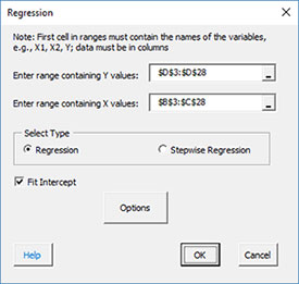
- Enter range containing Y values: the worksheet range containing the Y values
- Enter range containing X values: the worksheet range containing the X values
- Select the “Regression” option
- Fit intercept: default is that the intercept will be fitted; unchecking the box will set the intercept to 0.
- Options: contains additional residual options
- Selecting the Options button gives the input form below. The default residuals are checked. You can change those options or add additional output such as leverage.
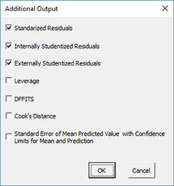
- Select OK to generate the regression analysis
- Select Cancel to exit the SPC for Excel program
Regression Output
There are four new worksheets added during the analysis:
- Data (1)
- Summary (1)
- Residuals (1)
- Regression Charts (1)
The number in parentheses is the number of regressions in the workbook. This allows you to keep track of the worksheets that go together when you remove observations, remove variables, or transform the Y variable and rerun the regression. The ranges containing the results on the first three sheets listed are protected. This is necessary for the program to find the information needed to rerun the regression. The four worksheets are described below.
Data
This worksheet contains the data used in the regression analysis.
Summary
The Summary worksheet is shown below. The regression model is shown at the top of the worksheet. This is followed by the ANOVA table for the model. If the model is statistically significant, the p value will be less than 0.05. If this is the case, the p value is shown in red. The predictor table is then shown. This contains the coefficients, standard error, t statistic, p value, VIF, and standardized coefficient. Coefficients with p values less than 0.05 are statistically significant. These will be in red also if they are less than 0.05.
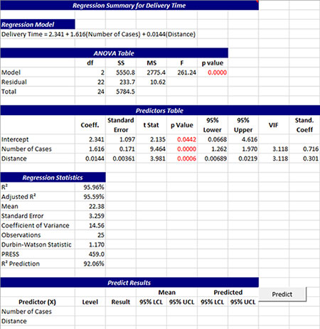
The regression statistics are then given. These include R Squared, adjusted R squared, the mean, standard error, coefficient of variance, the number of observations, the Durbin-Watson statistic, PRESS and the R squared prediction. The last part of the summary worksheet contains the section so you can predict results. The X values are listed in the first column. Enter levels for each predictor in the second column. Select “Predict” and the program will predict the result. It will also you provide 95% confidence limits for the mean at those levels, and 95% confidence limits for the predicted values.
Residuals
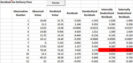
The residuals worksheet contains the observation number, the observed values, predicted values, and the residuals. The default residuals are the raw residuals, standardized residuals, internally studentized residuals, and externally studentized residuals. Potential outliers are shown in red. The “Revise” button on this worksheet is used to plot additional residual charts, remove observations, remove variables, or transform the y variables. See “Revising the Regression” below for more information.
Regression Charts
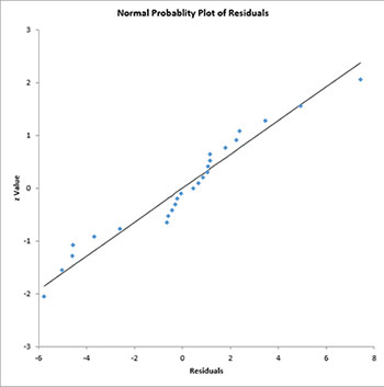
There are two charts that are automatically created in this worksheet: a normal probability plot for the residuals and the predicted values versus observed values chart.
The normal probability plot of the raw residuals is shown below. The residuals should fall around the straight line.
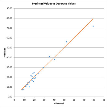
The predicted values versus observed values chart is shown below. A good model will have the points close to the line.
Additional charts are available from the “Revise” button on the residuals worksheet. See “Revising the Regression” below.
Revising the Regression
SPC for Excel allows you to add additional charts on the Regression Charts worksheet, or to revise the regression by removing observations, removing variables, or transforming the y variables. To access these options, select the “Revise” button on the residuals worksheet.
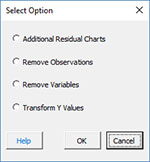
These four options are discussed below.
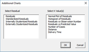
Additional Residual Charts
Selecting this option allows you to add additional charts via the form below. The residuals are listed on the left side (and will include leverage, etc. if those options were selected). You can select one type of residual. The possible X values are shown on the left-hand side. You may select multiple of these. Selecting OK will generate each chart selected, and place them on the Regression Charts worksheet.
Remove Variables
If you select the remove variable option, you will see the input screen below.

- Remove the variables selected in list box to the left: select the variables you want to remove in the list box shown; you may select more than one.
- Remove any variable with p value > 0.05: this option removes all variables with a p value greater than 0.05.
- Remove any variable with p value > 0.20: this option removes all variables with a p value greater than 0.20.
- Remove the variable with the highest p value: this option removes the variable with the largest p value.
- Remove any variable with p value > _: this option removes all variables with a p value greater than a value you enter.
Select OK and a new regression will be run.
Remove Observations
The residuals data worksheet contains information on the residuals. Some of the cells on this page may be in red representing possible outliers. The notes on the bottom of the page explain the outliers. If you want to remove some of these observations, select the Remove Observations option. You will get a box that lists all the observations. Select the observation(s) you want to delete and then select OK. A new regression will be run.
Transform Y Variable
You also have the option to transform the Y (response) value using some built in transformations. If you want to transform the Y values, select that option and the input screen below will be shown. Select the transformation option you want and a new regression will be run.