December 2015
 One of the many things we share in common is that we all live on this earth. And, according to the data, this earth of ours is getting warmer. This month (December 2015), almost 200 countries approved a climate accord that seeks to dramatically reduce emissions of greenhouse gases. These gasses are blamed by many for the increase in global temperatures that we have seen.
There are many climate models that are used to predict global temperatures in the future. These are, I am sure, very complex mathematical representations of the many interactions between the forces about our earth – oceans, land, atmosphere, our sun, etc. You don’t know how a model will perform in the future. So, scientists test the model to see how well it predicts the past.
That is the problem with data. It is all historical. Using historical data to predict the future of a complex variable like global temperatures is not easy. But like all analysis, it should begin by looking at the data over time.
This month’s publication takes a look at the annual average global temperature data from 1880 to 2015 through the use of control charts. The global temperature has not always been increasing during this time frame. It definitely has not been decreasing, but there appear to be six distinct time periods. Each of these time periods begins with a significant step change in the average global temperature.
This publication demonstrates how a control chart can be used to identify different periods of homogeneity in a set of data – periods of consistency and predictably. And from this consistency comes the ability to predict for the future.
So, instead of using all those fancy global warming models, we will use a simple control chart to predict the average global temperatures for 2015 and 2016.
In this issue:
- The Temperature Data
- The Run Chart
- 1880- 1894
- 1895- 1918
- 1919- 1935
- 1936- 1976
- 1977- 1997
- 1998- 2015
- Trends in Control Chart
- Prediction for 2015 and 2016
- Summary
- Quick Links
You may download a pdf version of this publication at this link. Please feel free to leave a comment at the end of the newsletter.
The Temperature Data
 The data used in this analysis covers the time period from 1880 through 2015 and was downloaded from the Goddard Institute for Space Studies (GISS) website at this link. GISS is part of the National Aeronautics and Space Administration (NASA). You can also download the data in an Excel workbook by selecting this link. The data includes monthly and annual data. Only the annual data are used in this publication. The data for 2015 contains the months of January through November.
(Update note 1/24/2016: Please note that the data used below are based on the meteorological station data, which is called the dTs data. There is also the LOTI (land, ocean, temperature index). According to the website, the LOTI provides a more realistic representation of the global mean trends than dTs below; it slightly underestimates warming or cooling trends, since the much larger heat capacity of water compared to air causes a slower and diminished reaction to changes; dTs on the other hand overestimates trends, since it disregards most of the dampening effects of the oceans that cover about two thirds of the earth’s surface.”)
The Run Chart
The data from 1880 to 2015 were first analyzed using a simple run chart – just plotting the data (in degrees Celsius) over time to see what it looks like. This chart is shown in Figure 1.
Figure 1: Run Chart for Annual Global Temperatures

Well, it is easy to see that the annual global temperature is definitely increasing over time. In fact, it looks like 2015 – the last point on the chart – will be the warmest year since 1880. Remember, the 2015 temperature in the run chart is based on the first 11 months of the year.
What else do you see in the chart? It does look like there are several fairly “level” global temperature periods – times when the global temperature was not increasing. We will use those “level” periods of times to build a control chart that shows a movie of global warming over time. This will help us find periods of homogeneity that can be used to predict the future.
1880- 1894
 The first “level” period of global temperature is at the beginning of the chart from 1880 to 1894. The data for this time period were used to construct an individuals control chart. With an individuals control chart, the individual value (annual global temperature) is plotted over time. The average is then calculated and added to the control chart. Then the lower control limit (LCL) and upper control limit (UCL) are calculated and added to the control chart. These control limits define the boundary of results when only common causes of variation are present – i.e., the normal variation in the process.
For more information, please see our publication on individual control charts and our publication on interpreting control charts.
The control chart for 1889 to 1894 is shown in Figure 2. The moving range control chart is not included in this analysis.
Figure 2: Global Temperatures for 1880 to 1894

The control chart is Figure 2 is in statistical control. There are no points beyond the control limits and no patterns – such as a run above the average – within the control limits. So, this was a period where the global temperature was not increasing but staying the same – averaging 13.52 °C.
Since the global temperature is in statistical control, we can predict what will happen in the future as long as the process stays the same. The global temperature will average 13.52 but could be as high as 13.87 (UCL) or as low as 13.17 (LCL). That is the normal variation in the global temperature process at that time.
The key phrase above is “as long as the process stay the same.” But, it didn’t. Something happened.
1895- 1918
The time period from 1895 to 1918 appears to be fairly level in terms of global temperatures. The average control limits from Figure 2 were set and then data from 1895 to 1918 were added to the control chart using the average and those control limits. This allows us to see any process changes. And did the process change! The control chart with the new data added is shown in Figure 3. What do you see?
Figure 3: Global Temperatures from 1880 to 1918

The control chart in Figure 3 is not in statistical control. Something happened to increase the global temperatures. There is a run of 10 years starting in 1895 above the average global temperature for the first part of the control chart. Then there is another run of 9 in a row above the average towards the end of the control chart.
To help see the magnitude of the change, the control limits can be split in 1895. This is shown in Figure 4.
Figure 4: Global Temperatures for 1880 to 1918 with Split Control Limits

Figure 4 shows that there was step change in global temperature starting in 1895, increasing the average from 13.52 to 13.68 – an increase of 0.16 °C. These data now represent the new norm – at least for that time period. What caused this step change to occur? Time for another step change.
1919 – 1935
The data from 1919 to 1935 is the next “level” period of temperature. This time period has been added to the data using the split control limit approach and is shown in Figure 5.
Figure 5: Global Temperatures from 1880 to 1935

Another step change for the period of 1919 to 1935 is apparent. The average temperature for this time period was 13.81 – an increase of 0.13 °C over the previous time period. What caused this step change to occur? Now for 41 years of consistent global temperature.
1936 – 1976
The 41-year period from 1936 to 1976 represents a long period where the global temperature did not increase or decrease – it just stayed the same. This time period has been added to the control chart and is shown in Figure 6.
Figure 6: Global Temperatures from 1880 to 1976
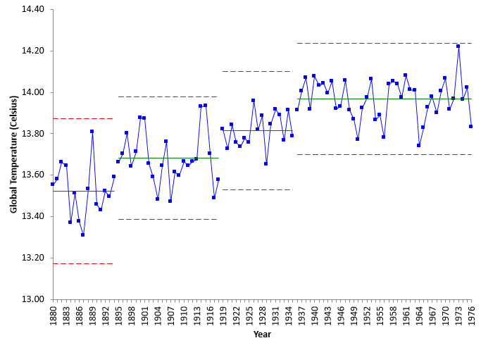
The average global temperature for this time period is 13.97 – an increase of 0.16 °C from the previous time period. But, for these 41 years, there is no evidence that the global temperature was increasing or decreasing.
 The four time periods considered so far have been periods of “level” global temperatures. If you regress the global temperatures versus the year numbers for each individual time period, you will find there are no significant correlations. For example, the p-value for the regression for the time period from 1936 to 1976 is 0.88 – nowhere near statistically significant. But you can see this in the way the global temperature bounces about the average for that time period as shown in Figure 6.
But, once again, something changes – and more dramatically – in 1977. The “level” periods of global temperatures appear to be going away.
1977- 1997
This 21-year period changes the way we have looked at the data so far. Yes, there is a step-change up, but for the first time, there is an indication that the temperature is not level during this time period but increasing. The data from 1977 to 1997 have been added to the control chart as shown in Figure 7.
Figure 7: Global Temperatures from 1880 to 1997

This time period has a larger step change than previous time periods. The average global temperature for 1977 to 1997 was 14.35 – an increase of 0.38 °C from the previous time period.
But look closely at the data plotted from 1977 to 1997. Most of the data starting in 1997 are below the average for the time period while most at the end of the time period are above the average. This is an indication that the temperature is increasing. If you do a regression analysis on the 1977 to 1997 data, you will find that there is a significant correlation between the year and the global temperature. The p value is less an 0.05 – which implies there is statistically significant relationship between the global temperature and the year number. The ANOVA table for this regression is shown in the table below.
| df | SS | MS | F | p value | |
| Model | 1 | 0.142 | 0.142 | 11.19 | 0.0034 |
| Residual | 19 | 0.241 | 0.0127 | ||
| Total | 20 | 0.382 |
The model (best-fit equation for the data) is given by:
Global Temperature = -12.606 + 0.0136(Year)
For the time period from 1997 to 1997, the global temperature increased an average of 0.0136 °C per year. The slope is the coefficient for the year number. Now for the last time period.
1998- 2015
There appears to have been another step change in the global temperature beginning in 1998 – in addition to the average yearly increase seen from 1977 to 1997. The time period from 1998 to 2015 has been added to the control chart as shown in Figure 8.
Figure 8: Global Temperatures 1880 – 2015

This time period has the highest step change. The average for the time period is 14.78 – a 0.43 °C increase from the previous time period. Once again, there appears to be indications that this is not a “level” period of global temperature, but a period of increasing global temperature.
A regression analysis was performed for the global temperature versus year number for the time period from 1998 to 2014. Note that the partial result for 2015 was not included in this regression. The ANOVA table for this regression is shown in the table below.
| df | SS | MS | F | p value | |
| Model | 1 | 0.0465 | 0.0465 | 5.72 | 0.0303 |
| Residual | 15 | 0.122 | 0.00812 | ||
| Total | 16 | 0.168 |
The p-value is 0.0303, which is less than 0.05. So, we conclude that there is significant relationship between the year and the global temperature.
The best fit regression equation is:
Global Temperature = -6.634 + 0.010672(Year)
From 1998 to 2014, the global temperature increased an average of 0.010672 °C per year – a little less than the previous time period.
So, there is a significant increase in global temperature each year during the last two time periods. The global temperature is not “level” during these two time periods. Does that mean our control chart approach fails? That the last two periods are not homogenous? Not at all.
Trends in Control Charts
![]() If there is a significant trend in the data, a trend control chart can be used to analyze the results. Take the last time period of 1998 to 2014. The regression analysis shows that the global temperature is increasing each year for that time period. Is the process in control during this time period?
If there is a significant trend in the data, a trend control chart can be used to analyze the results. Take the last time period of 1998 to 2014. The regression analysis shows that the global temperature is increasing each year for that time period. Is the process in control during this time period?
You can use best fit equation as the center line on the control chart and produce a trend control chart as shown in Figure 9. The control limits are still based on the average moving range and trend as the center line does.
Figure 9: Trend Control Chart for Global Temperatures from 1998 to 2014

This trend control chart is in statistical control. There are no points beyond the control limits and no patterns. Thus the data are homogeneous and can be used to predict the future – again as long as the process stays the same. For 2014, the value of the center line is 14.86, while UCL = 15.14 and LCL = 14.57.
2015 and 2016 Prediction
The control chart in Figure 9 can be used to predict the temperature for 2015 since it is in statistical control (again as long as the process stays the same).
Using the best-fit equation, the predicted temperature for 2015 is:
Global Temperature = -6.634 + 0.010672(Year) = -6.634 + 0.010672(2015) = 14.87
It could range between the upper and lower control, which will range from 14.59 to 15.15. The average temperature for the first 11 months of 2015 is 14.96. So, our estimate may be a little low, but it does appear to be within the control limits.
If we use 14.96 as the final average temperature for 2015 and re-run the regression, the trend control center line equation is:
Global Temperature = -9.8409 + 0.01227(Year)
The predicted value for 2016 is then:
Global Temperature = -9.8409 + 0.01227(2016) = 14.90
We will check back in a year and see how we did.
Summary
This publication has examined annual global temperatures from 1880 to 2015. Control charts were used to build a movie over time of how that temperature is changing. We found six distinct time periods where the data were homogeneous. The first four time periods were “level” temperature periods separated by step changes in the global temperature. The last two time periods were also homogenous and had the step change in temperature – but they were also characterized by statistically significant increases in temperature each year. The results are summarized below.
| Time Period | Average Temperature | Increase | Change per Year |
|---|---|---|---|
| 1880 – 1894 | 13.52 | 0 | |
| 1895 – 1918 | 13.68 | 0.16 | 0 |
| 1919 – 1935 | 13.81 | 0.13 | 0 |
| 1936 – 1976 | 13.97 | 0.16 | 0 |
| 1977 – 1997 | 14.35 | 0.38 | 0.0136 |
| 1998 – 2015 | 14.78 | 0.43 | 0.0107 |
It is interesting that there have been 6 step changes over time. What caused these step changes in average global temperatures? What is causing the yearly increase starting in 1977? It may well be greenhouse emissions. Maybe the topic for a future newsletter.