April 2009
In this issue:
- Yes/No Data: p and np Control Charts
- Binomial Distribution
- Counting Data: c and u Control Charts
- Poisson Distribution
- Small Sample Cases
- When to Use Each Chart
Last month we introduced the np control chart. With that publication, we have now covered the four attributes control charts. This month we review the four types of attributes control charts and when you should use each of them. We have now devoted one publication to each of the four control charts:
- p Control Charts
- np Control Charts
- c Control Charts
- u Control Charts
You can access these four publications at this link. These four control charts are used when you have “count” data. Sometimes this type of data is called attributes data. There are two basic types of attributes data: yes/no type data and counting data. The type of data you have determines the type of control chart you use. We hope you enjoy the newsletter!
Yes/No Data: p and np Control Charts
 With this type of data, you are examining a group of items. For each item, there are only two possible outcomes: either it passes or it fails some preset specification. Each item inspected is either defective (i.e., it does not meet the specifications) or is not defective (i.e., it meets specifications).
Suppose you teach a green belt workshop for your company. You have implemented a process that requires each participant to pass a written exam as well as complete a project in order to be given the title of green belt. This is yes/no type of data. Either a participant completes the requirement or does not complete the requirement.
Suppose one workshop has 20 attendees. This is the subgroup size (n). A “defective” participant is one who does not complete the requirements. The number of participants in the workshop who do not complete the requirements is denoted by np. Suppose that two participants do not complete the requirements, i.e., np = 2. The fraction defective is called p. In this example, p = np/n = 2/20 = .10 or 10% of the participants did not meet the requirements. As an instructor, you can track this data for each workshop.
There are two ways you can track the data: use the p control chart or the np control chart, depending on what you are plotting and whether or not the subgroup size is constant over time.
The p control chart plots the fraction defective (p) over time. The subgroup size does not have to be the same each time. This means that sometimes you can have 20 participants, another time 22, another time 18 and so on.
The np control chart plots the number defective over time, and the subgroup size has to be the same each time. This means you must have 20 participants each time, or you may take a random sample that is the same each time.
Binomial Distribution
The p and np control charts involve counts. You are counting items. To use the p or np control chart, the counts must also satisfy the following four conditions, as shown in Advanced Topics in Statistical Process Control (Dr. Don Wheeler, www.spcpress.com):
- The area of opportunity for defective items to occur must consist of n distinct items (e.g., there are 20 distinct participants in the workshop)
- Each of the n distinct items is classified as possessing or not possessing some attribute (e.g., for each student, determine if the requirements were met or not met)
- Let p be the probability that an item has the attribute; p must be the same for all n items in a sample (e.g., the probability of a participant meeting or not meeting the requirements is the same for all participants).
- The likelihood of an item possessing the attribute is not affected by whether or not the previous item possessed the attribute (e.g., the probability that a participant meets or does not meet the requirements is not affected by others in the group).
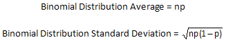
If these four conditions are met, the binomial distribution can be used to estimate the distribution of the counts; the p or the np control chart can be used. The control limits equations for the p and np control charts are based on the assumption that you have a binomial distribution. The binomial distribution is a distribution that is based on the total number of events (np) rather than each individual outcome. The average and standard deviation of the binomial distribution are given below:
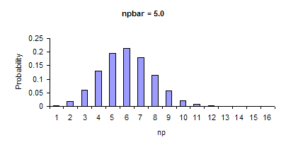
An example of a binomial distribution with an average number defective = 5 is shown below.
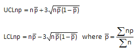
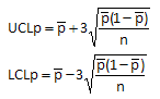
The control limits for both the np and p control charts are based on this distribution as can be seen below. The limits are based on the average +/- three standard deviations. The point to remember is that it is three standard deviations of the binomial distribution – not the standard deviation you get from calculating the standard deviation using something like Excel’s STDEV function.
np Control Chart: Control Limits
![]()
where k is the number of subgroups
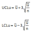
p Control Chart: Control Limits
Remember that to use these equations, the four conditions above must be met. Be careful here because condition 3 does not always hold. For example, some people use the p control chart to monitor on-time delivery on a monthly basis. A p control chart is the same as the np control chart, but the subgroup size does not have to be constant. You cannot use the p control chart unless the probability of each shipment during the month being on time is the same for all the shipments. Big customers often get priority on their orders. The probability of their orders being on time is different from that of other customers so you cannot use the p control chart. If the conditions are not met, consider using an individuals control chart.
Counting Data: c and u Control Charts
 We just looked at yes/no type of data that classifies an item as defective or not defective. If the item is complex in nature, like a television set, computer or car, it does not make much sense to characterize it as being defective or not defective. For example, a television set may have a scratch on the surface, but that defect hardly makes the television set defective. The real issue here is how many defects there are on the television set.
Rating items as defective or not defective is also not very useful if the item is continuous. For example, suppose you are making a plastic sheet. The fact that the sheet has a small defect such as a bubble or blemish on it does not make it defective. However, if there are too many bubbles, the sheet may not be useful for its intended purpose.
For example, suppose you make plastic sheets that are used for sheet protectors. Bubbles on the plastic sheet are considered defects. You can monitor the number of bubbles over time by counting the number of bubbles on one plastic sheet. The plastic sheet is the area of opportunity for defects to occur. The number of bubbles is the number of defects (c).
A defect occurs when something does not meet a preset specification. It does not mean that the item itself is defective. When looking at counting data, you end up with whole numbers such as 0, 1, 2, 3; you can’t have half of a defect. Thus, with the plastic sheet example, you will have 1 bubble, 2 bubbles, etc.
There are two ways to track this counting type data, depending on what you are plotting and whether or not the area of opportunity for defects to occur is constant.
The c control chart plots the number of defects (c) over time. The area of opportunity must be the same over time. This means that you use the same sized sheet each time you are counting the bubbles in the sheet.
The u control chart plots the number of defects per inspection unit (c/n) over time. The area of opportunity can vary over time. This means that you can vary the number of sheets or the area examined for bubbles each time.
Poisson Distribution
There are four conditions that must be met to use a c or u control chart. These are listed in Advanced Topics in Statistical Process Control (Dr. Wheeler, www.spcpress.com) as follows:
- The counts must be discrete counts (e.g., each bubble that occurs is discrete).
- The counts must occur in a well-defined region of space or time (e.g., one plastic sheet is the well-defined region of space where the bubbles can occur).
- The counts are independent of each other, and the likelihood of a count is proportional to the size of the area of opportunity (e.g., the probability of finding a bubble on a plastic sheet is not related to which part of the plastic sheet is selected).
- The counts are rare compared to the opportunity (e.g., the opportunity for bubbles to occur in the plastic sheet is large, but the actual number that occurs is small).
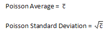
If these conditions are met, then the Poisson distribution can be used to model the process. This distribution is used to model the number of occurrences of a rare event when the number of opportunities is large but the probability of a rare event is small. The average and standard deviation of the Poisson distribution are given below:
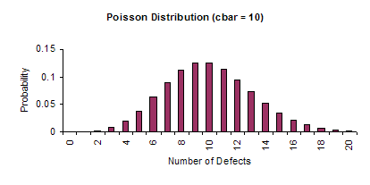
An example of the Poisson distribution with an average number of defects equal to 10 is shown below.
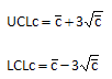
The control limits for both the c and u control charts are based on the Poisson distribution as can be seen below. The limits are based on the average +/- three standard deviations. The point to remember is that it is three standard deviations of the Poisson distribution – not the standard deviation you get from calculating the standard deviation using something like Excel’s STDEV function.
c Control Chart: Control Limits
u Control Chart: Control Limits
Remember that the four conditions above must be met if you are going to use these control limit equations to model your process. If the conditions are not met, consider using an individuals control chart.
Small Sample Cases
The control limits given above are based on either the binomial or the Poisson distribution. The conditions listed above for each must be met before they should be used to model the process. However, there is a time when the control limit equations do not apply. If the n * average fraction defective is less than 5, the control limits above for the p and the np control charts are not valid. The control limits for the c and u control charts are not valid if the average number of defects is less than 3. For more information on this, please see the two newsletters below:
Small Sample Case: p and np Control Charts
Small Sample Case: c and u Control Charts
There is also more information on the binomial and Poisson distributions in those two newsletters.
When to Use Which Chart
The table below shows when to use each of the charts. X-mR is the individuals control chart.
| Yes/No Data | Counting Data |
||||||
| Subgroup size = n | Area of Opportunity = n | ||||||
| Follows Binomial Distribution? | Follows Poisson Distribution? | ||||||
| Yes | No | Yes | No | ||||
| Constant n | Variable n | X-mR Chart | Constant n | Variable n | X-mR Chart | ||
| np Chart | p Chart | c Chart | u Chart | ||||
More information on the individuals control chart can be found here. It is important to remember that the assumptions underlying the control charts are important and must be met before the control chart is valid.
Summary
This month’s publication reviewed the four basic attribute control charts: p, np, c and u. The equations for the average and control limits were given as well as the underlying assumptions for each type of control chart. When to use each chart was introduced.