Keeping the Process on Target: CUSUM Charts

August 2014

This month’s publication explores the one-sided cumulative sum (CUSUM) control chart.   The primary purpose of a CUSUM control chart is to detect small shifts from the process target.  Over the years, our publications have covered a number of different control charts.  These charts are primarily Shewhart control charts, e.g., X-R, X-s, and X-mR control charts.  These types of control charts are very useful in monitoring a process for statistical control or to see the impact of your process improvement efforts.  You can also increase the sensitivity of these charts by using the zone tests and run tests in addition to the points beyond the control limits test for out of control conditions.

The CUSUM control chart approach is different.  The major aims of the CUSUM control chart is to keep the process on target.  The “cumulative sum” in this type of chart is the sum of the deviations of individual sample results or subgroup averages from the target.  The CUSUM control chart plots these cumulative deviations over time and will indicate when the process is “out of control” – or in this case, significantly off-target.

In This Issue:

• Introduction to CUSUM control charts
• The Data Set
• Analysis Using Shewhart Control Chart
• Analysis Using CUSUM Control Charts
• Comparing the Two Approaches
• Summary
• Quick Links

Click here to download a pdf file of this publication.

Introduction to CUSUM Control Charts

Like all control charts, a CUSUM control is a method of looking at your process variation.  A CUSUM control chart monitors the deviations of individual samples results (X values) or subgroup averages (X values) from a target value.  The target value is the same as your process aim – where you want the process to operate.  The cumulative sum is the sum of these deviations over time.

To use a CUSUM control chart, you have to answer two basic questions.

1. What shift from the target do you want to be able to detect?

This shift is usually ½ or 1 standard deviation of the parameter being plotted.  Thus, the data helps you set the shift to detect.  This shift is often referred to as the “allowable slack” in the process.

2. Where do you want the action limits set?

The action limits are similar to control limits.  The standard practice is to set these actions at 4 times the standard deviation.  Again, the data helps set the action limits.

It is clear you will need a method of estimating the standard deviation of the process.  This is covered below.

A CUSUM control chart then tracks the deviations from the target.  If a sample result is within the allowable slack, the process is considered to be operating on target.  This results in a subtraction from the cumulative sum unless it is already zero.   If a sample result is beyond the allowable slack, the process is considered to be operating off target.  This results in an addition to the cumulative sum.  If the cumulative sum exceeds the action limits, the process is assume to be off target.

There are two “one-side” cumulative sums.  One for deviations that are positive (above the target) and one for deviations that are negative (below the target).  Let’s take a look at an example to see how this works.  We will compare the results when using an individuals control chart to using the CUSUM control chart.

The Data Set

You are producing a chemical that contains a small amount of component Y that is important in the use of the chemical.    In addition, you know that the optimum concentration for that component is 0.16 wt. %.  You want to control the manufacturing process as close to that as possible.  You take a sample every batch.  The results for the last 25 batches are shown below.

Table 1: The Data Set

Analysis Using Shewhart Control Chart

Since our batch data represents one data point at a time, an individuals control chart (X-mR) can be used to monitor the results.  This is the most common way the data would be analyzed.  But remember, the purpose of a Shewhart control chart is primarily to keep the process in control and to see the impact of process improvement efforts.  With a CUSUM control chart, you are trying to detect small shifts away from the process target.

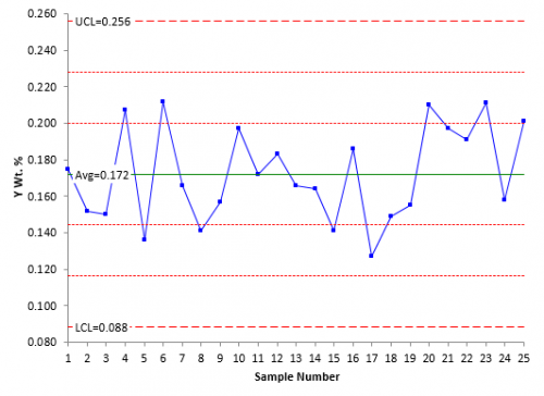
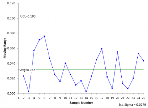
The data in Table 1 were analyzed using the X-mR chart.   Please see our October 2006 publication for more information on X-mR charts. Figure 1 shows the X chart.  This chart monitors the variation in the individual results over time.  Figure 2 shows the moving range (mR) chart.  This chart monitors the variation in the range between consecutive samples.

Figure 1: X Chart for Y Wt. %

Figure 2: mR Chart for Y Wt. %

The X chart is in statistical control.  There are no points beyond the limits and there are no issues with the zone tests or run tests.   The process average is 0.172.  This is different from the process target of 0.166.  But not by much.  Is it significantly different?  The individual results can vary between the lower control (LCL) of 0.088 and the upper control limit (0.256).  The process is consistent and predictable.

Note that 5 out of the last 6 points are above average.  Is this a problem?  Under the classical control chart approach, it is not a problem.  There is not enough evidence of you to assume that a special cause of variation exists and spend time looking for that special cause.  For more information on interpreting control charts, please see our April 2004 publication.

The mR chart is in statistical control as well.   The average moving range between consecutive samples is 0.032.  It can be as great as the UCL of 0.103.  Since the range chart is in control, you can estimate the process standard deviation from the range chart.  Remember above where we said you needed a standard deviation (s).  This is where you get it.  For the X-mR chart, the standard deviation is given by the following:

s =R /1.128 = 0.0279

Analysis Using CUSUM Control Charts

Let’s take a look at the data using a CUSUM control chart.  The first step is to determine the standard deviation of the data.  This is used to set the allowable slack and the action limits.  The best way to estimate the standard deviation is from a range control chart.  For the individuals control chart, this is the moving range chart where sigma is estimated from the average range.  As shown above, the estimate of the standard deviation is 0.0279.

The next step is to determine the allowable slack (k).  It is common to set this value at ½ to 1 standard deviation.  We will use ½.   So,

k = 0.5(0.0279) = 0.01395

The next step is to determine the action limits (H).  These are usually set as +/- 4 sigma. So,

H =+/- 4(0.0279) = +/- 0.1116

The next step is to calculate the cumulative sums on the high side (SH, above the target) and on the low side (SL, below the target).  We know that our target is 0.16.   The following are the definitions for SH and SL.

SH(i)= Max[0, SH(i-1) + X_i – Target – k]

SL(i) = Min(0, SL(i-1) + X_i – Target + k]

where

• i = i^th sample
• SH(i) is the high side cumulative sum for the i^th point
• SH(i-1) is the high side cumulative sum for the i^th – 1 point
• X_i is the result for the i^th point
• Target = target value
• k = allowable slack
• SL(i) is the low side cumulative sum for the i^th point
• SL(i-1) is the low side cumulative sum for the i^th – 1 point

Take a look at the equation for SH(i).  It contains:

X_i  – Target – k = X_i – (Target + k)

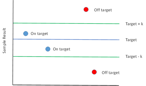
So, if X_i > (Target + k), then the i^th sample result is outside the allowable slack range on the high side.

Similarly, for SL(i):

X_i – Target + k = X_i – (Target – k)

So, if X_i < (Target – k), then the i^th sample result is outside the allowable slack range on the low side.  Figure 3 shows this.

Figure 3: On or Off Target

Let’s see how the calculations unfold.  Note that the equations for SH and SL include the i^th and i^th -1 results for SH and SL.  What about the first sample?  There is no sample before the first sample.    For the first sample, SH(0) = 0 and SL(0) = 0.

The first sample result is 0.175.  Note that this result is above our aim of 0.16.  If it is far enough away, then it should add to the high side value of SH.

SH(1)= Max[0, SH(0) + 0.175 – 0.16 – 0.01395] = Max[0, 0.001] = 0.001

SL(1) = Min(0, SL(0) + 0.175 – 0.16 + 0.01395] = Min[0, 0.029] = 0

The second sample result is 0.152.  Note that this result is below our aim.  It if is far enough away, then it should add to the low side value of SL.

SH(2)= Max[0, 0.001 + 0.152 – 0.16 – 0.01395] = Max[0, -0.021] = 0

SL(2) = Min(0, 0 + .152 – 0.16 + 0.01395] = Min[0, .00595] = 0

Table 2 shows the results of the calculations for all 25 samples.   Note that both SH and SL return to zero several times.

Table 2: CUSUM Calculation Results

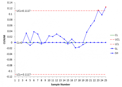
Remember that our action limits are +/- 0.1116.  This value is exceeded by SH(23), our 23rd sample.  This tells us that the process has moved significantly off target and needs to be adjusted to return the process to the target value.

You could simply use this tabular form for the cumulative sum.  However, it is better to chart the results.  Figure 4 is a plot of the CUSUM chart.

Figure 4: CUSUM Chart

The center line on the CUSUM chart is zero.  Both the SH and SL values are plotted.  You can see how the cumulative sums on the high side begin to pile up around sample 20 and continue until the action limit is exceeded.

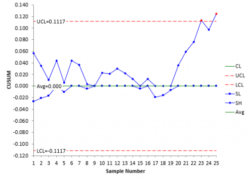
Once the process has been adjusted back to target, the values of SH and SL are set back to zero.  However, there is technique called Fast Initial Response (FIR) in which the values are not set back to zero, but are set to certain value, usually 2 standard deviations.  This provides a method of responding faster to off-target operations.  You can also start a CUSUM chart with a FIR.  Figure 5 shows that results where the FIR method is used to initialize the chart.

Figure 5: CUSUM Chart with FIR Initialization

You can see from this chart that both SH and SL are further away from 0 than in Figure 4.  If the process is off target, then the CUSUM control chart will pick it up faster.  If it is on target, the CUSUM values will trend back to zero as shown in the middle of the chart.

You can estimate the current process average when a point exceeds the action limits.  In this example, that occurred at sample 23 and it occurred on the high side.  The following can be used to estimate the current process average.

Current process average = Target + k + (SH/NH)

where SH = value of SH when the action limit was exceeded and NH = the number of consecutive points above 0 when the action limits were exceeded.  You can see in Figure 4 and Figure 5 that the 23rd result is the fourth point in a row above 0.  So, NH = 4.  With SH(23) = 0.113,

Current process average = .16 + 0.01395 + (0.113/4) = 0.202

If the action limit on the low size is exceeded, you find the current process average using:

Current process average = Target – k – (SL/NL)

where SL is the value of SL when the action limit was exceeded and NL is the number of consecutive points below 0 when the action limit was exceeded.

Comparing the Two Approaches

We examined the data using the individuals control chart and the CUSUM control chart.   Did the two charts give us the same information?  No, the individuals control chart indicated that the process was in statistical control.  As of yet, there is no indication that anything has changed in the process.  On the other hand, the CUSUM control chart indicated that the process had drifted off target on sample 23.  So, it picked up the change quicker than the classical control chart.

But remember: the two types of control charts have different purposes.  With the individuals control chart, the primary purposes are to keep the process in statistical control and to see the impact of process improvement efforts.  All processes will have drift in the average.  If small shifts in the average aren’t critical to you, the individuals control chart is fine.  It serves it purpose.  However, if there is little room for error and it is more important that the process operate on target, then consider using the CUSUM control chart.  Note that if there is a true shift in the process average, the individuals control chart will pick it up eventually.

One of the biggest disadvantages of the CUSUM control chart is that the underlying data is lost.  You are not looking at actual values.  The individuals control chart gives you a picture of what is happening in the process through the use of actual values.  The CUSUM control chart is the sum of deviations – more difficult to see the underlying process behavior.  And for the most part, if you use the additional tests for out of control (zone tests, etc.) with the individuals control chart, the ability of the individuals control chart to detect small shifts approaches that of the CUSUM control chart.

Note that there are other control schemes for the CUSUM control chart.  These schemes are based on the ARL – the average run length.  ARL is the average number of samples required before an out of control situation occurs.  To minimize the number of false out of control points, the ARL should be large when the process is operating on target.  It should be small if the process average has shifted off target.  Different values of k and H create different ARL.  Using k = 0.5 and H = 4 provides a CUSUM control chart that has good ARL for a shift in process average of one standard deviation.  For more information, please see “Introduction to Statistical Quality Control” by Douglas C. Montgomery.  You can also search online for “CUSUM ARL” to find more information.   The ARL is based on a point beyond the action or control limits.

Summary

This publication has introduced the one-sided CUSUM control chart.  This type of control chart monitors the cumulative sum of deviations from the process target.  It is designed to detect small shifts in the process average from the target value.  It is called “one-sided” because there is a cumulative sum on the high side (above the target) and a cumulative sum on the low side (below the target).  You can adjust the CUSUM ability to detect shifts by changing the values of k (the allowable slack) and H (the action limits).  This type of chart will detect the process shift much quicker than waiting for a point beyond the control limits for the individuals control chart.  However, applying the zones tests to the individuals control chart improves its ability to detect those small shifts.