January 2010
This is a first in a series of newsletters designed to introduce experimental design techniques. We will be looking at two-level full factorial designs. There are many types of experimental designs but you can accomplish a lot with two-level designs.
The newsletter series will show you how to plan, conduct and analyze these two level designs. A manual method of analyzing the results is given. This manual method provides clear method of understanding what an effect is, what a main effect is and what an interaction between factors is. We will use ANOVA (analysis of variance) in a later newsletter to analyze experimental design results. This is the most common way of examining the results of an experimental design with software that is available today.
In this first newsletter, we will cover the following:
- Introduction to the design problem
- Experimental design terminology
- Experimental design data
- Effects and main effects
- Interaction between factors
- Are the main effects and interactions significant?
- Quick Links
Introduction to the Problem
Suppose your process involves a stirred batch reactor. Your product is a chemical and the purity of that chemical is critical to customers. You would like to improve the chemical’s purity. There are two process variables that you think impact the purity: the reactor temperature and the residence time of the chemical in the reactor. How do you find out the following?
- Do the reactor temperature and/or residence time impact the average purity
- If so, by how much? For example, if I change the reactor temperature 5 degrees, what is the impact on the average purity?
- Do the reactor temperature and/or residence time impact the variation in the purity?
- If so, by how much? For example, if I increase the residence time in the reactor by 10 minutes, do the purity results have more variation?
Experimental design techniques can help you quickly find out the answers to these questions. Some people still approach experiments doing the “one factor at a time” approach. If you use this approach, you would change reactor temperature while holding residence time constant. Once you found the optimal purity, you would then hold the reactor temperature at that level and change residence time. The one factor approach is not efficient and does not account for interaction between reactor temperature and residence time as we will see in this series of newsletters. We begin by introducing the terminology associated with experimental design.
Experimental Design Terminology
There are various terms that are widely used with experimental design techniques. These terms are introduced below.
An experimental design is a planned experiment to determine, using a minimum number of experimental runs, what factors have a significant effect on a product response and/or variability in the product response and how large the effect is in order to find the optimum set of operating conditions. In this example, our experimental design is a planned experiment that is used to determine how reactor temperature and residence time affect purity so we can find the optimum operating conditions.
A factor is a variable over which there is direct control. It is the independent variable in statistical terms. In this example, we have two factors: the reactor temperature and the residence.
The level of a factor refers to the value of the factor used in an experimental run. The levels of residence time are 30 minutes and 90 minutes. The levels of temperature are 50°C and 90°C.
Qualitative factors are factors whose levels can not be arranged in magnitude of order. Examples include different shifts or different operators in a plant. Quantitative factors are factors whose levels can be arranged in order of magnitude. Reactor temperature and residence time are examples of quantitative factors.
Fixed factors are factors whose levels in an experiment are set at particular values. Both factors in our example are fixed. There are also random factors. Random factors are factors whose levels in an experimental run are only randomly chosen samples from a population of levels that could be included. For example, a raw material may contain an impurity that may affect your process. Although you do not have direct control over the impurity, you can randomly select two different samples of the raw material. The impurity is then a random factor.
A response is a variable whose value depends upon the levels of the factors. It is the dependent variable in statistical terms. In this example, purity is the response.
A discrete response is one that does not produce a numerical value. This type of response produces attributes data: yes/no or counting. A continuous response does produce a numerical value. Purity is a continuous response.
Experimental Design Data
Two factors, reactor temperature and residence time, are thought to impact the product purity obtained in a chemical reaction. A planned experiment to investigate this could take the form shown below.
| Residence Time | Temperature | |
| t0 = 50°C | t1 = 90°C | |
| r0 = 30 minutes | Cell 1 | Cell 2 |
| (Three runs) | (Three runs) | |
| r1 = 90 minutes | Cell 3 | Cell 4 |
| (Three runs) | (Three runs) | |
A treatment or treatment combination is represented by one cell. For example, in cell 1, the treatment is temperature = 50°C and residence time = 30 minutes. A treatment represents the levels of all factors used in a given experimental run. For this experimental design, there are four treatments (r0t0, r0t1, r1t0, and r1t1).
Each treatment combination is run three times. This is called replication of the treatment. In total, we have 12 experimental runs. Suppose we have conducted these experimental runs in random order. The results are shown below. The table also shows the average as well as the range (maximum – minimum) for each treatment combination.
| Run | Rx. Temp. | Res. Time | % Purity | Average | Range | ||
| 1 | 50 | 30 | 74 | 78 | 73 | 75 | 5 |
| 2 | 90 | 30 | 65 | 64 | 69 | 66 | 5 |
| 3 | 50 | 90 | 74 | 76 | 78 | 76 | 4 |
| 4 | 90 | 90 | 85 | 88 | 91 | 88 | 6 |
Experimental error is represented by the difference in experimental runs with the same factor levels. For example, the run number 1 was replicated three times. The differences (74, 78, and 73) in the purity for these two run is caused by experimental error. Experimental error is not a very good term for this. It is actually measuring the process variation. This process variation will be used to determine if a factor has a significant effect on a response. If the differences seen in the response variable due to different levels of the factor can be explained by normal process variation, we will conclude that the factor does not affect the response. However, if the differences can not be explained by normal process variation, we will conclude that the factor does affect the response.
Effects and Main Effects
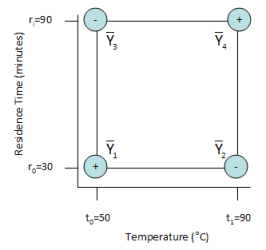
The concepts of effects, main effects and interactions are introduced below. The two factor design above can be drawn as shown below.
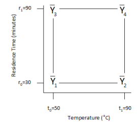
The bars over the Y mean that it is an average value. The subscripts represent the run number from above. A subscript of 1 is the average purity (the response variable) for all experimental runs made at the treatment with residence time = 30 minutes and temperature = 50°C (r0t0 treatment). Likewise, the subscript 2 is the average purity at treatment r0t1, the subscript 3 is the average purity at treatment r1t0, and the subscript 4 is the average purity at treatment r1t1.
An effect is defined as the average response when a factor is at its high level minus the average response when a factor is at its low level with all other factors held constant. There are four effects that can be determined in this example. The effect of temperature when residence time is at its low level (30) can be determined as shown in the figure below.
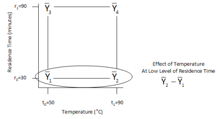
The effect of temperature at the low level of residence time is the difference between the average of the runs labeled “Run 2” and the average of the runs labeled “Run 1” in the results table above.
![]()
This means that the average purity decreases by 9 when temperature is increased from 50 to 90 when the residence time is at 30.
The effect of temperature at the high level of residence time is given by:
![]()
The effect of residence time at low level of temperature is given by:
![]()
The effect of residence time at high level of temperature is given by:
![]()
This experimental design provides estimates of four effects. This is one reason experimental design techniques are so powerful.
An effect takes into account only the change in the response variable when one factor is changed from its high to low level with all other factors constant. The main effect takes into account the different levels of the other factors.
A main effect is defined as the difference between the results when a factor is at its high level and when a factor is at its low level. For example, the main effect of temperature is the average of the results when temperature is at its high level minus the average of the results when temperature is at its low level. The figure below uses a plus sign (+) to indicate the high level of a factor and a minus sign (-) is used to indicate a low level of a factor. As you can see, the main effect of temperature is the average of the runs 2 and 4 minus the average of runs 1 and 3.
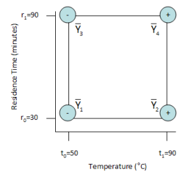
Algebraically, the main effect of temperature is given by:
![]()
This means that the average purity increases by 1.5 as the reactor temperature increases from its low level to its high level.
The main effect for residence time can be viewed as the average of the results when residence time is at its high level minus the average of the results when residence time is at its low level as shown in the figure below. The main effect of residence time the average of runs 3 and 4 minus the average of runs 1 and 2.

Algebraically, the main effect of residence time is given by:
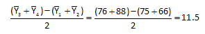
This means that the average purity increases 11.5 as residence time increases from its low level to its high level.
Interactions Between Factors
The main effect describes how a factor influences a product response. This influence, however, sometimes depends on the levels of the other factors. This is called interaction. For example, the effect of temperature on purity may vary when residence time is at its low level from when residence time is at its high level.
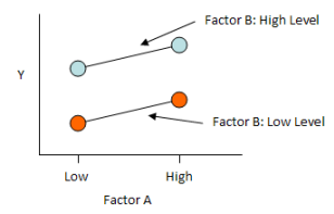
There are three possible types of interactions. These are easy to see if you plot the response variable (Y) versus the two factors. The figure below is an example of no interaction. Factor A is on the x axis; the response variable on the Y axis. The two lines represent the results for Y when Factor B is at its high level (blue) and when Factor B is at its low level (red). The two lines are essentially parallel. This means there is no interaction between the factors.
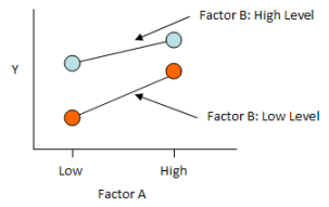
The second type of interaction is shown in the figure below. The lines are no longer parallel. There is a moderate interaction between the factors. The effect of temperature on Y is stronger when Factor B is at its low level than when Factor B is at its high level.
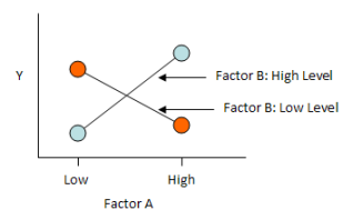
The third type of interaction is a strong interaction. This is shown in the figure below. When Factor B is at its low level, Y decreases as Factor A increases. But when Factor B is at its high level, Y increases as Factor B increases.
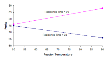
In the reactor example, there is a strong interaction between reactor temperature and residence time as shown in the plot below. When residence time is at 30 minutes, increasing reactor temperature decreases purity. But when residence time is at 90 minutes, increasing temperature increases purity.
Algebraically, the interaction between temperature and residence time is defined as the average of the effect of residence time at the high level of temperature minus the average of the effect of residence time at the low level of temperature:
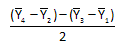
It should be noted that the same equation is obtained if the interaction is defined as the average of the effect of temperature at the high level of residence time minus the average of the effect of temperature at the low level of residence time.
The above equation for the interaction can be rewritten as:
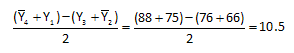
As seen in this equation, the interaction can be viewed as the average difference in results obtained at the corners of the square as shown in the figure below.
Are the Effects, Main Effects and Interactions Significant?
Experimental design techniques are used to determine the main effects and interactions. We have determined the following so far:
- Main Effect of Temperature = 1.5
- Main Effect of Residence Time = 11.5
- Interaction between Temperature and Residence Time = 10.5
Are these numbers significant? If a factor does not have an effect on a product response, one would expect the main effect or interaction to be zero. Of course, with normal process variation, the main effect or interaction will not be zero. For a main effect or interaction to be statistically significant, it must be significantly different from zero. Next month’s newsletter will describe how to determine if these main effects or interaction are statistically significant.