May 2013
 We hear a lot about government spending these days – not just in the United States but in just about every country around the world. Here in the United States, our two political parties snap at each other every single day. The Republicans say that President Obama and the Democrats spend way too much money and we are too far in debt. And the Republicans say they gave in to raising taxes so that door is closed in the future. President Obama and the Democrats say that they have already cut spending and that the Republicans are blocking their ability to reduce the deficit by blocking tax increases on the wealthy and corporations. And the Democrats say that the rate of spending increases has declined. So, who is correct? Well, it depends how you spin it, and our politicians are the pros at spinning things.
It is amazing how often people simply listen to their favorite news source and then assume what they hear is correct. They might hear: “Spending is way up under President Obama” from a Fox News analyst. Or they might hear: “President Obama has cut spending” from an ABC news analyst. Of course, this makes it easy on a person – no thinking, no checking for the facts – simply listen to what someone says or read what they wrote and assume you are getting the facts. It takes a little work to delve into the facts.
Often though, it is quite simple. You can learn a lot by merely plotting the data over time. Many times, you don’t need to make a statistical control chart to see what is happening – a run chart will tell you a lot. This month we will take a look at the United States government – how much money is spent and how large our deficit is. We will start with a run chart and then move to analysis through a control chart. Fun and games ahead.
In this Issue:
- The Time Period Considered and the Data
- Government Spending
- Government Spending and Control Charts (1977 – 2001)
- Government Spending and Control Charts (1977 – 2008)
- Government Spending and Control Charts (1977 – 2012)
- The Deficit
- Summary
- Quick Links
Feel free to leave a comment at the end of the newsletter.
The Time Period Considered and the Data
 In analyzing data, you have to make a decision about how far back to go in time. We chose to go back to 1977, the first year Jimmy Carter was President of the United States. Since 1977, we have had three Republican presidents (Reagan, Bush and Bush) and three Democratic presidents (Carter, Clinton and Obama). We didn’t get into our financial problems overnight and, the fact that both parties have been represented in the White House over the past 35 years, shows there is plenty of blame to go around.
The data included in the analysis are the yearly expenditures and the yearly deficits. These data are available from the White House web at the time this was written. Since the population has been increasing in the United States over time, we also decided to look at government spending per capita. The data for the United States population came from this link. The data are shown in the table below – along with who was president at the time. The outlays per capita are given in $ per person, while receipts, outlays, deficit and population columns represent millions.
Table 1: United States Government Spending
| Millions | ||||||
| Year | President | Receipts | Outlays | Deficit | Population | Outlays per Capita |
| 1977 | Carter | 355,559 | 409,218 | -53,659 | 219.75987 | $ 1,862 |
| 1978 | Carter | 399,561 | 458,746 | -59,185 | 222.09508 | $ 2,066 |
| 1979 | Carter | 463,302 | 504,028 | -40,726 | 224.56724 | $ 2,244 |
| 1980 | Carter | 517,112 | 590,941 | -73,830 | 226.54581 | $ 2,608 |
| 1981 | Reagan | 599,272 | 678,241 | -78,968 | 229.46571 | $ 2,956 |
| 1982 | Reagan | 617,766 | 745,743 | -127,977 | 231.66446 | $ 3,219 |
| 1983 | Reagan | 600,562 | 808,364 | -207,802 | 233.79199 | $ 3,458 |
| 1984 | Reagan | 666,438 | 851,805 | -185,367 | 235.8249 | $ 3,612 |
| 1985 | Reagan | 734,037 | 946,344 | -212,308 | 237.9238 | $ 3,978 |
| 1986 | Reagan | 769,155 | 990,382 | -221,227 | 240.13289 | $ 4,124 |
| 1987 | Reagan | 854,288 | 1,004,017 | -149,730 | 242.28892 | $ 4,144 |
| 1988 | Reagan | 909,238 | 1,064,416 | -155,178 | 244.49898 | $ 4,353 |
| 1989 | G. Bush | 991,105 | 1,143,744 | -152,639 | 246.81923 | $ 4,634 |
| 1990 | G. Bush | 1,031,958 | 1,252,994 | -221,036 | 249.4644 | $ 5,023 |
| 1991 | G. Bush | 1,054,988 | 1,324,226 | -269,238 | 252.15309 | $ 5,252 |
| 1992 | G. Bush | 1,091,208 | 1,381,529 | -290,321 | 255.0297 | $ 5,417 |
| 1993 | Clinton | 1,154,335 | 1,409,386 | -255,051 | 257.78261 | $ 5,467 |
| 1994 | Clinton | 1,258,566 | 1,461,753 | -203,186 | 260.32702 | $ 5,615 |
| 1995 | Clinton | 1,351,790 | 1,515,742 | -163,952 | 262.80328 | $ 5,768 |
| 1996 | Clinton | 1,453,053 | 1,560,484 | -107,431 | 265.22857 | $ 5,884 |
| 1997 | Clinton | 1,579,232 | 1,601,116 | -21,884 | 267.78361 | $ 5,979 |
| 1998 | Clinton | 1,721,728 | 1,652,458 | 69,270 | 270.248 | $ 6,115 |
| 1999 | Clinton | 1,827,452 | 1,701,842 | 125,610 | 272.69081 | $ 6,241 |
| 2000 | Clinton | 2,025,191 | 1,788,950 | 236,241 | 282.19216 | $ 6,339 |
| 2001 | G. W. Bush | 1,991,082 | 1,862,846 | 128,236 | 285.10208 | $ 6,534 |
| 2002 | G. W. Bush | 1,853,136 | 2,010,894 | -157,758 | 287.94122 | $ 6,984 |
| 2003 | G. W. Bush | 1,782,314 | 2,159,899 | -377,585 | 290.78898 | $ 7,428 |
| 2004 | G. W. Bush | 1,880,114 | 2,292,841 | -412,727 | 293.6554 | $ 7,808 |
| 2005 | G. W. Bush | 2,153,611 | 2,471,957 | -318,346 | 296.50706 | $ 8,337 |
| 2006 | G. W. Bush | 2,406,869 | 2,655,050 | -248,181 | 299.39848 | $ 8,868 |
| 2007 | G. W. Bush | 2,567,985 | 2,728,686 | -160,701 | 301.62116 | $ 9,047 |
| 2008 | G. W. Bush | 2,523,991 | 2,982,544 | -458,553 | 304.05972 | $ 9,809 |
| 2009 | Obama | 2,104,989 | 3,517,677 | -1,412,688 | 307.00655 | $ 11,458 |
| 2010 | Obama | 2,162,706 | 3,457,079 | -1,294,373 | 309.33022 | $ 11,176 |
| 2011 | Obama | 2,303,466 | 3,603,059 | -1,299,593 | 311.59192 | $ 11,563 |
| 2012 | Obama | 2,450,164 | 3,537,127 | -1,086,963 | 313.91404 | $ 11,268 |
Government Spending
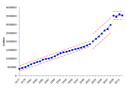
 It is usually a little difficult to tell what is happening just from a table of numbers. But if you look at the column called “Outlays”, a fancy name for spending our tax dollars, you can easily see that it has increased a lot over the past 35 years. It is still worth just charting the outlays over time to easily see the magnitude of the change over that time. This is done in Figure 1.
Figure 1: Government Spending (1977 – 2012)
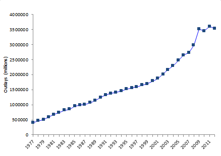
Wow – a large increase over time, from about 400 billion in 1977 to 3.5 trillion in 2012. No doubt about it – government spending has been increasing over the years. That is kind of expected since we have had inflation and more people for the government to handle. We will ignore inflation but will take a quick look at population growth.
Figure 2 shows the government spending per capita (per person). It looks essentially the same as Figure 1 – definitely increasing over time. Our population increases and the government continues to spend more money per person. In 2012, our government spent over $11,000 per person. What do you see in Figures 1 and 2?
Figure 2: Government Spending per Capita (1977 – 2012)
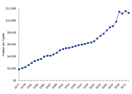
You can see three stages in government spending in either chart. We will use a control chart to examine these three different stages. One stage covers the period of 1977 to 2001, where the upward trend in spending seems to be at one level; then from 2002 to 2008 where the upward trend increases to a higher level, and then from 2009 on where the spending appears to have leveled off – but at a huge spending level!
Government Spending and Control Charts (1977 – 2001)
Can you use a control chart with the data in Figures 1 and 2? Yes, you can, but it is not the classical control chart because the data are trending upward. You need to use a trend control chart. Let’s return to the data in Figure 1, the outlays. We will break the chart into three stages based on events that have occurred. The first stage covers the time period from 1977 through 2001. This trend control chart is shown in Figure 3.
Figure 3: Trend Control Chart for Government Spending (1977 to 2001)
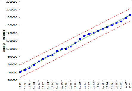
Figure 3 is a trend control chart based on individual yearly spending values. With a trend control chart, the center line is the best fit line. This is determined by regression. The best fit line for these data are:
Spending = 59789(Year) – 117950458
We did not include the moving range chart here, but the average moving range is used to determine how far the control limits are from the best fit line. The control limits are set at +/-2.66 times the average moving range. As long as there are no points beyond the control limits or any patterns (like seven points in a row above or below the best fit line), the process is in statistical control.
This chart is in statistical control. It says that, on average, the outlays have increased by 59,789 million (or about 60 billion) per year since 1977. This is the slope of the best fit line. And since the chart is in statistical control, we can expect that trend to continue as long as the process stays the same. However, the process changed as we will see below.
The chart shows that spending increased through each president’s term during this time period. This includes President Reagan, who was known for pushing for smaller government. The fact is that government spending did increase under his presidency from 1981 to 1988. But it has increased for all presidents since 1977 (and before that as well). Now let’s take a look at what happened after 2001.
Government Spending and Control Charts (1977 – 2008)
Figure 4 shows a control chart based on the data from 1977 through 2008. The control chart shows a break in the year 2002. This is because the process changed with the 9/11 attack in 2001. The government increased spending on anti-terrorist measures and on the two wars in Iraq and Afghanistan.
Figure 4: Trend Control Chart for Government Spending (1977 to 2008)
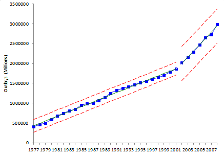
The time period from 2002 through 2008 shows increased spending. The best fit line for that time period is:
Spending = 157669(Year) – 313654721
The slope of this line is almost 158 billion. This means that during this time period, the average increase in spending each year was 158 billion, almost three times the amount of during the time frame from 1977 to 2001. So, yes spending did increase significantly during this time frame under George W. Bush. But, the greatest jump in spending was yet to come.
Government Spending and Control Charts (1977 – 2012)
This now brings us to the Obama years. The run chart in Figure 1 shows the jump in spending that occurred in 2009 when Obama took office. Or course, the Democrats blame Bush for this saying his fiscal policies caused the banking and housing crisis of 2008. The Republicans blame it on the Democrats and their inability to address the housing issue and the large increases in spending on the social programs. Probably Bush and Obama can share the responsibility for this spending increase.
But the chart also shows something else – four years in a row that spending appears to have leveled off – something that had not happened in the previous 30 plus years. Figure 5 shows the control chart with this third stage added.
Figure 5: Trend Control Chart for Government Spending (1977 to 2012)
So, what can you say about government spending. Under all presidents since 1977, government spending has increased (giving Obama partial credit for the spending increase in 2009), but since 2009, spending has leveled off – we aren’t spending more – but we sure are spending at the highest level in the history of this country. Spending went down slightly in 2010 and 2012 and up some in 2013 – but that appears to be normal variation now.
So, the Republicans are right – the government under Obama is spending more than ever in the past. And the Democrats are right – spending has decreased under Obama during two years – and the rate of spending has decreased significantly – to about zero the past three years. It is all in how you spin the data. What about the deficit? Well, see below.
The Deficit
So did the deficit soar as government spending increased from 1977 to 2012? Let’s take look.
Figure 6 shows the deficit over this time period.
Figure 6: Deficit per Year (1977 – 2012)
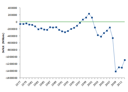
The run chart shows that there has been a deficit for all but the time frame from 1998 to 2001 (the Clinton years as the Democrats like to remind people). Starting in 1991, there was a nice upward trend in deficit reduction (started in the Bush years, continuing through the Clinton years). Then the deficit increased after 9/11 and then had a sharp increase with the banking and housing problems of 2008 and beyond.
The chart helps see the magnitude of the change in deficit – a real and scary problem for the United States and for many countries around the world. Just about everyone knows you can’t sustain a system where more goes out than comes in over the long run. It would be nice if our politicians worked together to solve the problem and not just blame the other side and hope to make it to the next election cycle. And that goes for politicians in both parties! But just plotting the data over time shows the magnitude of the change – helping one see the true changes in the process. Most of us have a hard time with billions of dollars, let alone trillions.
Summary
 You can learn a lot by simply plotting data over time – you don’t always need to do a control chart. Just seeing how the data arises over time will give you a much deeper insight into the underlying process than if you just looked at a table of numbers – or worse, relied on some news organization to tell you what the data means when they seldom know how to look at data and draw rational conclusions. A picture is worth a thousand words. Just plot the data – it is so simple!
An ending quote often attributed to another Illinois Senator of 50 years ago, Everett Dirksen:
“A billion here, a billion there, pretty soon, you’re talking real money.”
And this was back in the 1950s and 1960s!
Dear Bill,If I had the power, I would nominate you for the Nobel Prize! Your newsletters are simply brilliant. They explain stats in such a simple practical manner. Keep up the good work. Best regards, Shankar ShridharMelbourne, Australia
Hi everyone,Another way to look at this would be to not stage the last 4 data points, then only 2009 would show as an exceptional increase, the remaining data points staying within the limits of stage two.Take care not to stage just to tell "your" story or to "fit" the data!Best regardsPierre
Hi Pierre,Thanks for the comment. Yes, I thought about looking at the data without the third stage. Actually, if you base the limits on the 2002 to 2008 data as a trend chart, then 2009 data point is just below the UCL. The other three remain within the those limits as you state. The reason I didn't do that was because there was a process change that year with the increase in spending to bail out the banks (among other items). And the results in spending from that year onward represent the first time spending has not increased each year – so that trend was broken. It may not have failed one of the classical test for out of control, but that appeared to me to be a significant process change. So, that is why I went with the third stage.
Hi Bill,Would you please explain how you managed to get the trend lines in figure 3 ? Regards, Rahul
The calculations for the trend control chart are the same for the individuals chart except for the average line. The value of the average line is the best fit line: Y = b1X + b0 where b1 and b0 are constants determined by regression. Y is the center line (X double bar), e.g., the spending for that year; and X is the year.<br /><br />So,<br />UCL = Y + 2.66Rbar = b1X + b0 + 2.66Rbar LCL = Y – 2.66Rbar = b1X + b0 – 2.66Rbar<br />where Rbar is the average moving range of 2.