January 2013
This is the first of a multi-part newsletter on rational subgrouping – a very important, yet often forgotten, part of statistical process control (SPC). Far too often, people do not give enough (or any) thought about how to subgroup their data when constructing an X-R control chart or any other control chart that involves putting the data into subgroups. One needs to remember that control charts are really a study of the variation in your process. And the variation displayed on the control chart depends on how you subgroup your data – which may or may not be the variation you would like to study. We will use the sport of golf to help us explore rational subgrouping in this newsletter.
In this issue:
- Rational Subgrouping
- Golf and Rational Subgrouping
- Golf Data
- Golf and Control Charts
- Phil Mickelson
- Summary
- Quick Links
As always, please feel free to leave a comment at the end of the newsletter.
Rational Subgrouping
So, what is rational subgrouping? Lloyd Nelson defined rational subgrouping as “a sample in which all of the items are produced under conditions in which only random effects are responsible for the observed variation” (Control Charts: Rational Subgroups and Effective Applications, Journal of Quality Technology, Vol. 20, No. 1, Jan. 1988). This is the premise behind rational subgrouping – the results that are combined into the same subgroup can be logically thought to have been obtained or produced under essentially the same conditions. We will start our discussion of rational subgrouping by considering the sport of golf. This analogy will help us see how rational subgrouping works – and give us more insight into understanding how X-R control charts work.
Golf and Rational Subgrouping
 Golf is a great game – at least some folks think so. Imagine that you are a pro golfer – getting to fly around the world to beautiful golf courses throughout the year and compete for million dollar purses in golf tournaments. Golf tournaments consist of four rounds of 18 holes of golf played over four days. So, suppose you are a golf pro – like Phil Mickelson. You want to monitor whether your golf score is getting better. How could you do this?
One method would be to track your average tournament score, i.e., the average of the four rounds. You would like to see this score get lower since lower scores improve your ability to earn money in the pros. You would also probably be interested in your consistency, i.e., how close the four rounds in a tournament are. You won’t like a lot of variation your results – shooting a 72 one day and a 90 the next. So, you could also track the range in your golf scores for a tournament. The perfect chart to do this is the X-R control chart.
Like all control charts, the X-R control chart examines variation. To use an X-R control chart, you need to determine how to subgroup the data. You should never just take the existing data and put it into a subgroup size of 4 or 5 simply because you read that most of the time a subgroup size of 4 or 5 is used with the X-R control chart. It makes sense (one of the tenets of rational subgrouping), with golf, to subgroup the data by tournament. The four rounds of golf for a single tournament form a subgroup. This will allow us to explore the variation we are interested in: our average score and our consistency.
Golf Data
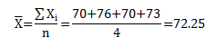
Suppose the first tournament you play for the year has the following results for the rounds: 70, 76, 70, and 73. Pretty nice four rounds of golf for you! These four rounds form the first subgroup. You can calculate the subgroup average (the average of the four rounds of golf):
You can continue this for each tournament you are in and plot the results on an X control chart. This chart shows you have much variation there is in your average tournament score from tournament to tournament – this is the variation between subgroups and is sometimes called the long-term variation.
You can also calculate the range of this first tournament of the year (the first subgroup). The range is simply the highest score (76) minus the lowest score (70). So, the range for the first subgroup is:
Range = Highest – Lowest = 76 – 70 = 6
You are pretty consistent! You can continue this for each tournament you are in and plot the results on the R chart. This chart shows you how much variation there is in your scores within a tournament from tournament to tournament – this is the variation within a subgroup and is sometimes called the short-term variation.
Table 1 shows your scores for your last 18 tournaments. The tournament (subgroup) averages and ranges have also been calculated. The overall average for the 18 tournaments and the average range have also been calculated as shown in the table.
Table 1: Tournament Scores
|
Tourn. No. |
Round 1 |
Round 2 |
Round 3 |
Round 4 |
Average |
Range |
|
|
1 |
70 |
76 |
70 |
73 |
72.25 |
6 |
|
|
2 |
72 |
66 |
71 |
73 |
70.5 |
7 |
|
|
3 |
68 |
67 |
69 |
71 |
68.75 |
4 |
|
|
4 |
68 |
68 |
72 |
67 |
68.75 |
5 |
|
|
5 |
71 |
69 |
72 |
68 |
70 |
4 |
|
|
6 |
71 |
67 |
75 |
77 |
72.5 |
10 |
|
|
7 |
69 |
76 |
70 |
71 |
71.5 |
7 |
|
|
8 |
67 |
71 |
67 |
67 |
68 |
4 |
|
|
9 |
70 |
68 |
71 |
68 |
69.25 |
3 |
|
|
10 |
70 |
71 |
66 |
74 |
70.25 |
8 |
|
|
11 |
67 |
71 |
70 |
69 |
69.25 |
4 |
|
|
12 |
75 |
66 |
73 |
73 |
71.75 |
9 |
|
|
13 |
73 |
71 |
70 |
75 |
72.25 |
5 |
|
|
14 |
66 |
68 |
71 |
78 |
70.75 |
12 |
|
|
15 |
73 |
69 |
73 |
67 |
70.5 |
6 |
|
|
16 |
69 |
65 |
67 |
76 |
69.25 |
11 |
|
|
17 |
72 |
71 |
70 |
67 |
70 |
5 |
|
|
18 |
69 |
72 |
68 |
74 |
70.75 |
6 |
|
|
Sum |
1266.25 |
116 |
|||||
|
Average |
70.34722 |
|
One key to understanding X-R control charts is to understand that the two charts are monitoring different sources of variation. The X control chart is examining the variation in subgroup averages over time and will let you know if these subgroup averages are consistent (in control – only common causes of variation present) or if any subgroup averages fall outside the “normal” variation (out of control – special cause of variation present). The R chart is examining the variation within the subgroup over time and will let you know if this within subgroup variation is consistent over time. If you are new to control charts, please review our newsletter on the purpose of control charts.
Golf and Control Charts
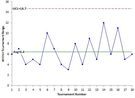
As mentioned before, the subgroup averages are plotted on the X control chart and the subgroup ranges are plotted on the R chart. Figure 1 is the X run chart for these 18 tournaments. Figure 2 is the R chart for the tournaments. The averages are plotted on each chart as well, but the control limits have not yet been added.
Figure 1: X Run Chart for Golf Data
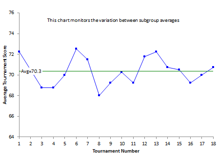
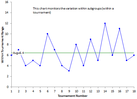
Figure 2: R Run Chart for Golf Data
Whenever you look at a control chart, the first question you should ask yourself is
“What variation is this chart examining?”
If you can’t answer this question, then the control chart is nonsense – it will not tell you anything at all. Throw it out and start over with a discussion of rational subgrouping. Figure 1 is measuring the variation in tournament averages from tournament to tournament. You can see this because you are plotting the tournament averages over time. In control chart language:
“The X control chart is monitoring the variation in the subgroup averages from subgroup to subgroup.”
Figure 2 is measuring the variation within the four rounds in a single tournament from tournament to tournament. You are plotting this range (the maximum minus the minimum value) over time. In control chart language:
“The R chart is monitoring the variation within the subgroup from subgroup to subgroup.”
The next step is to add the control limits. The control limits for the X and R control charts are shown below.
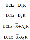
where D4, D3, and A2, are control chart constants that depend on subgroup size (see our newsletter on X-R control charts). Our subgroup size in this case is 4, since there are four rounds per tournament. R is the average on the range chart and ![]() is the average of the X control chart.
is the average of the X control chart.
One important item to note on the control limits: the average range is used in the calculation of the control limits for the X control chart. This means that the “short-term” variation from the range chart is used to set the control limits for the “long-term” variation on the X control chart. We will come back to this point next month.
Figure 3 is the X control chart with the control limits added. Figure 4 is the R chart with the control limits added.
Figure 3: X Control Chart for Golf Data
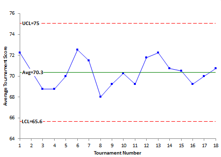
Figure 4: R Control Chart for Golf Data
Remember that the upper control limit (UCL) represents the largest value we would expect from the process if there are only common causes of variation present. In this example, the UCL = 75.04. This means that the highest tournament average one would expect is 75 as long as only common causes of variation are present. The LCL represents the smallest value we would expect from the process if only common causes of variation are present. The LCL = 65.61. This means the smallest tournament average we would expect is about 65.6 as long as only common causes of variation are present.
As long as there are no points beyond the control limits and no patterns, the X control chart is in statistical control. This is the case as seen in Figure 3. This means that the variation in the subgroup averages (tournament averages) is consistent over time. The process is consistent and predictable. It means that we can predict what will happen in the future. We don’t know what the next tournament average will be, but we do know that it will be between 65.61 and 75.04 with a long term average of 70.32 as long as the process stays the same. It also tells us that our golf score is not getting lower over time.
Figure 4 is the range chart with the control limits added. Remember that this chart is monitoring the variation in the range of scores from a single tournament. The average range (6.47) is the centerline on the chart. The upper control limit (14.77) is also plotted. In this example, there is no lower control limit. Since there are no points beyond the control limits or patterns, the R chart is in statistical control. This means that we can predict what will happen in the future. We don’t know the exact range of scores that will occur in the next tournament, but we do know that it will vary between 0 and 14 with a long term average of 6.47 as long as the process stays the same.
Once a process is in statistical control, the only way to improve it is to fundamentally change the process. If we want our average score to decrease or to be more consistent, we have to change the way we do things. Fundamental changes could include a different golf coach, a new swing, or new clubs.
Phil Mickelson
The tournament scores in Table 1 look like they were made by a pretty good golfer. They were. The data are the PGA tournament scores for Phil Mickelson in 2010. He was pretty consistent in 2010. How has he been since then?
Table 2 shows his PGA tournament rounds for those tournaments where he made the cut from 2010 through 2012. He did not miss the cut on too many tournaments. The data are from www.espn.com.
Phil turned pro in 1992. He is 42 years now. He made $4.2 million in 2012 on the tour. Not bad! The control charts based on the data in the table are shown below.
Table 2: Phil Mickelson Golf Scores
| Date | PGA Tournament (Tour) | Tourn. No. | Round 1 | Round 2 | Round 3 | Round 4 |
| Jan 28 – 31 (2010) | Farmers Insurance Open | 1 | 70 | 76 | 70 | 73 |
| Feb 4 – 7 | Northern Trust Open | 2 | 72 | 66 | 71 | 73 |
| Feb 11 – 14 | AT&T Pebble Beach National Pro-Am | 3 | 68 | 67 | 69 | 71 |
| Feb 25 – 28 | Waste Management Phoenix Open | 4 | 68 | 68 | 72 | 67 |
| Mar 11 – 14 | WGC-CA Championship | 5 | 71 | 69 | 72 | 68 |
| Mar 25 – 28 | Arnold Palmer Invitational | 6 | 71 | 67 | 75 | 77 |
| Apr 1 – 4 | Shell Houston Open | 7 | 69 | 76 | 70 | 71 |
| Apr 8 – 11 | The Masters | 8 | 67 | 71 | 67 | 67 |
| Apr 29 – May 2 | Quail Hollow Championship | 9 | 70 | 68 | 71 | 68 |
| May 6 – 9 | THE PLAYERS Championship | 10 | 70 | 71 | 66 | 74 |
| Jun 3 – 6 | the Memorial Tournament | 11 | 67 | 71 | 70 | 69 |
| Jun 17 – 20 | U.S. Open Championship | 12 | 75 | 66 | 73 | 73 |
| Jul 15 – 18 | The Open Championship | 13 | 73 | 71 | 70 | 75 |
| Aug 5 – 8 | WGC-Bridgestone Invitational | 14 | 66 | 68 | 71 | 78 |
| Aug 12 – 15 | PGA Championship | 15 | 73 | 69 | 73 | 67 |
| Sep 3 – 6 | Deutsche Bank Championship | 16 | 69 | 65 | 67 | 76 |
| Sep 9 – 12 | BMW Championship | 17 | 72 | 71 | 70 | 67 |
| Sep 23 – 26 | THE TOUR Championship | 18 | 69 | 72 | 68 | 74 |
| Jan 27 – 30 (2011) | Farmers Insurance Open | 19 | 67 | 69 | 68 | 69 |
| Feb 3 – 7 | Waste Management Phoenix Open | 20 | 67 | 65 | 71 | 71 |
| Feb 10 – 13 | AT&T Pebble Beach National Pro-Am | 21 | 71 | 67 | 69 | 71 |
| Feb 17 – 20 | Northern Trust Open | 22 | 71 | 70 | 74 | 68 |
| Mar 10 – 13 | World Golf Championships-Cadillac Championship | 23 | 73 | 71 | 72 | 76 |
| Mar 24 – 27 | Arnold Palmer Invitational presented by Mastercard | 24 | 70 | 75 | 69 | 73 |
| Mar 31 – Apr 3 | Shell Houston Open | 25 | 70 | 70 | 63 | 65 |
| Apr 7 – 10 | The Masters | 26 | 70 | 72 | 71 | 74 |
| May 5 – 8 | Wells Fargo Championship | 27 | 69 | 66 | 74 | 69 |
| May 12 – 15 | THE PLAYERS Championship | 28 | 71 | 71 | 69 | 72 |
| Jun 2 – 5 | The Memorial Tournament | 29 | 72 | 70 | 72 | 67 |
| Jun 16 – 19 | U.S. Open Championship | 30 | 74 | 69 | 77 | 71 |
| Jul 14 – 17 | The Open Championship | 31 | 70 | 69 | 71 | 68 |
| Aug 4 – 7 | World Golf Championships-Bridgestone Invitational | 32 | 67 | 73 | 71 | 72 |
| Aug 11 – 14 | PGA Championship | 33 | 71 | 70 | 69 | 70 |
| Aug 25 – 27 | The Barclays | 34 | 67 | 70 | 68 | 68 |
| Sep 2 – 5 | Deutsche Bank Championship | 35 | 70 | 73 | 63 | 69 |
| Sep 15 – 18 | BMW Championship | 36 | 72 | 73 | 71 | 75 |
| Sep 22 – 25 | TOUR Championship by Coca-Cola | 37 | 68 | 70 | 67 | 71 |
| 1/19 – 1/22 (2012) | Humana Challenge | 38 | 74 | 69 | 66 | 69 |
| 2/2 – 2/5 | Waste Management Phoenix Open | 39 | 68 | 70 | 67 | 73 |
| 2/9 – 2/12 | AT&T Pebble Beach National Pro-Am | 40 | 70 | 65 | 70 | 64 |
| 2/16 – 2/19 | Northern Trust Open | 41 | 66 | 70 | 70 | 71 |
| 3/8 – 3/11 | World Golf Championships-Cadillac Championship | 42 | 72 | 71 | 71 | 71 |
| 3/22 – 3/25 | Arnold Palmer Invitational | 43 | 73 | 71 | 71 | 72 |
| 3/29 – 4/1 | Shell Houston Open | 44 | 65 | 70 | 70 | 71 |
| 4/5 – 4/8 | The Masters Tournament | 45 | 74 | 68 | 66 | 72 |
| 5/3 – 5/6 | Wells Fargo Championship | 46 | 71 | 72 | 68 | 71 |
| 5/10 – 5/13 | THE PLAYERS Championship | 47 | 71 | 71 | 70 | 73 |
| 5/17 – 5/20 | HP Byron Nelson Championship | 48 | 70 | 69 | 69 | 66 |
| 6/14 – 6/17 | U.S. Open Golf Championship | 49 | 76 | 71 | 71 | 78 |
| 8/2 – 8/5 | World Golf Championships-Bridgestone Invitational | 50 | 71 | 69 | 73 | 71 |
| 8/9 – 8/12 | PGA Championship | 51 | 73 | 71 | 73 | 74 |
| 8/23 – 8/26 | The Barclays | 52 | 68 | 74 | 67 | 76 |
| 8/31 – 9/3 | Deutsche Bank Championship | 53 | 68 | 68 | 68 | 66 |
| 9/6 – 9/9 | BMW Championship | 54 | 69 | 67 | 64 | 70 |
| 9/20 – 9/23 | TOUR Championship by Coca-Cola | 55 | 69 | 71 | 72 | 69 |
| 11/1 – 11/4 | World Golf Championships-HSBC Champions | 56 | 66 | 69 | 66 | 68 |
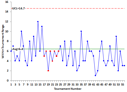
Figures 5 and 6 show the X and R control charts with the control limits based on the 2010 data. Still a pretty consistent golfer! Note that in Figure 6, there is a run of 8 points below the average. Something happened to make his game more consistent from that point on. We should probably re-calculate the control limits from that point on. But I will leave that to Phil. Or, if you would like to do it, e-mail me and I will send you the data in an Excel workbook.
Figure 5: Phil Mickelson X Control Chart
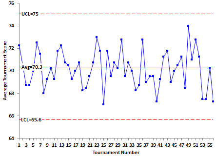
Figure 6: Phil Mickelson R Control Chart
Summary
Rational subgrouping provides the context you use to interpret a control chart. The first question you ask yourself when examining a control chart is “What variation is this chart examining?” This is the key to using control charts effectively. Without effective rational subgrouping, control charts can be simple nonsense.
We used the X-R control chart in this newsletter. The X-R control chart is a powerful tool for examining sources of variation but it is critical to set up the chart to explore the variation you are interested in. In this golf example, we were interested in monitoring our average tournament score as well as our consistency. The chart we used was setup to examine that variation. Note that, if we had plotted each individual tournament result, we would have been looking at different sources of variation. This is the principle behind rational subgrouping.
Next month we will take a more in-depth look at rational subgrouping including some rules to follow.