October 2019
(Note: all the previous SPC Knowledge Base in the variable control charts category are listed on the right-hand side. Select this link for information on the SPC for Excel software.)

In this issue:
- Introduction to the T2 Control Chart
- Constructing a T2 Control Chart
- Out of Control Points
- Summary
- Quick Links
You may download a pdf copy of this publication at this link. Please feel free to leave a comment at the end of the publication.
Introduction the T2 Control Chart
In 1947, Harold Hotelling introduced a statistic which allowed multivariate observations to be plotted on a single chart. This statistic is now called Hotelling’s T2 statistic. The statistic combines information from the mean as well as the dispersion of more than one variable. The calculations, which include some matrix algebra, are more difficult than those of “normal” control charts. This was a barrier to using multivariate control charts until software that could perform the calculations came along.
The T2 control chart is used to detect shifts in the mean of more than one interrelated variable. The data can be in subgroups (like the X-R control chart) or the data can be individual observations (like in the X-mR control charts).
A few words of caution. The T2 control chart, like other multivariate control charts, plots a value on the chart that you really can’t explain too well. Suppose you have two variables that are important in an adhesive process. The adhesive is characterized by two variables, pH and viscosity, which need to be controlled. Data for 20 batches are shown below for pH and viscosity. The data in this example is adapted from “Advanced Topics in Statistical Process Control” by Donald Wheeler (www.spcpress.com).
Table 1: pH and Viscosity Data
| Batch | pH | Viscosity | Batch | pH | Viscosity | |
|---|---|---|---|---|---|---|
| 1 | 7.75 | 5.48 | 11 | 8.30 | 5.58 | |
| 2 | 8.50 | 5.98 | 12 | 8.15 | 5.44 | |
| 3 | 7.50 | 4.12 | 13 | 8.20 | 3.11 | |
| 4 | 8.25 | 5.34 | 14 | 7.70 | 4.34 | |
| 5 | 7.50 | 4.36 | 15 | 7.55 | 4.08 | |
| 6 | 7.60 | 4.26 | 16 | 8.50 | 5.96 | |
| 7 | 7.90 | 4.50 | 17 | 8.20 | 5.80 | |
| 8 | 8.10 | 5.16 | 18 | 8.55 | 5.94 | |
| 9 | 8.10 | 5.56 | 19 | 7.65 | 4.00 | |
| 10 | 7.70 | 4.08 | 20 | 8.40 | 5.86 |
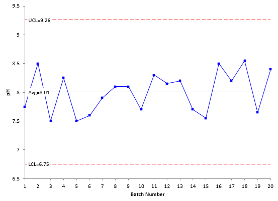
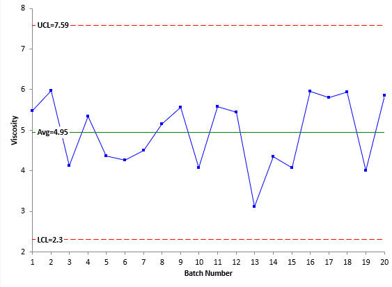
One way of monitoring the pH and the viscosity is by using a control chart for each variable. An individuals chart (X-mR) could be used for both pH and the viscosity. Figure 1 is the X chart for pH and Figure 2 is the X chart for viscosity. The moving range charts are not shown here.
Figure 1: X Chart for pH
Figure 2: X Chart for Viscosity
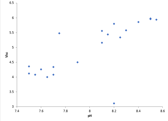
Figures 1 and 2 are both in statistical control. Look at the figures again. Notice anything? The two figures have very similar patterns. This implies that the two variables are correlated. A scatter diagram for the two variables is shown in Figure 3.
Figure 3: Scatter Diagram of pH vs Viscosity
The scatter diagram shows that the two variables are related. As pH increases, the viscosity tends to increase. Note the point at the bottom of the scatter diagram for a pH of 8.2. This data pair looks like it might be an outlier, despite the X charts being in control. This is where the T2 control chart can be used. It is designed to see the impact of multiple variables at the same time.
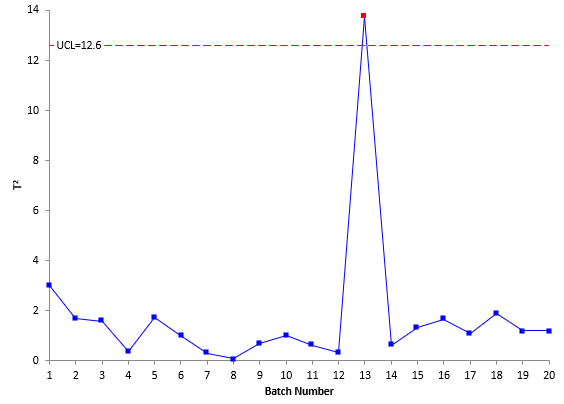
Figure 4 is the T2 control chart for the data in Table 1.
Figure 4: T2 Control Chart for pH and Viscosity
The T2 control chart shows an out of control point for batch 13. That out of control point does correspond to the low point on the scatter diagram above.
Look at the T2 control chart in Figure 4. One of the first things you may notice about this control chart is that the value of T2 has no resemblance to the original pH and viscosity data. So, looking at the value of T2 really tells you nothing about the original data.
The only test for out of control points on this type of chart is points beyond the upper control limit (UCL). There is no lower control limit (LCL). There is one point beyond the control limit – but you don’t know which variable (pH or viscosity) caused the out of control point by looking at the control chart. Information on how to determine which variable(s) is responsible is given below.
Constructing a T2 Control Chart
As stated before, the T2 control chart can be used with data in subgroups or data that are individual observations. We will use individual observations to show how to construct a T2 control chart. Note that the calculations are different for data in subgroups.
The first step in creating a T2 control chart is to calculate the values of T2. This is where matrix algebra comes in. The value of T2 is given by:
T2 = (x–x)‘S-1(x –x)
where x is the sample mean vector and S is the sample covariance vector. The bolded characters represent vectors. This is clearly now a little more complicated than the calculations for the basic control charts, but we will give you the general idea of how it is done for the case of two variables.
We will start with the(x–x)term in the T2 equation. To create this term, you subtract the average value for the variable from each individual value for the variable. The average for pH and viscosity are given below.
x for pH = 8.005
x for viscosity = 4.9475
From Table 1, the first point for pH and viscosity are 7.75 and 5.48 respectively. Then, for the first point,
This will be eventually calculated for each point. Note that it is a matrix with one row for each point and a column for each variable.
Now, (x–x)’is the transpose of (x–x). The transpose of (x–x) is:
The transposed matrix has a column for each point and a row for each variable.
The S matrix is a little more difficult to find. It is found from the vector of moving differences for each variable. For each variable, vi is found where
vi = xi+1 – xi
So, for pH, v1 is the difference between the second pH value and the first pH value:
v1 = 8.50 – 7.75 = 0.75
This is done for both variables and the vector V contains the results for both variables:
where m = number of samples. The components of V are given below for the two variables.
| pH | Viscosity |
|---|---|
| 0.75 | 0.5 |
| -1 | -1.86 |
| 0.75 | 1.22 |
| -0.75 | -0.98 |
| 0.1 | -0.1 |
| 0.3 | 0.24 |
| 0.2 | 0.66 |
| 0 | 0.4 |
| -0.4 | -1.48 |
| 0.6 | 1.5 |
| -0.15 | -0.14 |
| 0.05 | -2.33 |
| -0.5 | 1.23 |
| -0.15 | -0.26 |
| 0.95 | 1.88 |
| -0.3 | -0.16 |
| 0.35 | 0.14 |
| -0.9 | -1.94 |
| 0.75 | 1.86 |
So V has a column for each variable and m – 1 rows. S can now be found using the following:
where V’ is the transpose of V. You can easily multiply two matrices in Excel using the function MMULT. If you multiply V’ by V, you get the following:
S is then found by dividing each term in V’V by 2(m – 1) = 2(19) = 38.
Remember that T2 is given by:
T2= (x–x)‘S-1(x–x)
S-1 is the inverse of S. You can use the Excel function MINVERSE to find the inverse. Using that function gives:
Now we have all three terms:(x–x)‘,S-1, and(x–x)
So, for the first point:
T2= (x–x)‘S-1(x–x)
You can use the Excel MMULT function to multiply these three matrices together. The result is given below.
T2 = 3.006896
This is the value of T2 for the first data point. The above process can be used to generate the T2 values for the rest of the data. The values of T2 are shown in the table below.
Table 2: Values of T2 for pH and Viscosity
| Batch | pH | Viscosity | T2 | Batch | pH | Viscosity | T2 | |
|---|---|---|---|---|---|---|---|---|
| 1 | 7.75 | 5.48 | 3.006896 | 11 | 8.30 | 5.58 | 0.609407 | |
| 2 | 8.50 | 5.98 | 1.674520 | 12 | 8.15 | 5.44 | 0.324114 | |
| 3 | 7.50 | 4.12 | 1.580571 | 13 | 8.20 | 3.11 | 13.748666 | |
| 4 | 8.25 | 5.34 | 0.371990 | 14 | 7.70 | 4.34 | 0.614283 | |
| 5 | 7.50 | 4.36 | 1.734041 | 15 | 7.55 | 4.08 | 1.333028 | |
| 6 | 7.60 | 4.26 | 1.019390 | 16 | 8.50 | 5.96 | 1.648693 | |
| 7 | 7.90 | 4.50 | 0.292941 | 17 | 8.20 | 5.80 | 1.076091 | |
| 8 | 8.10 | 5.16 | 0.065993 | 18 | 8.55 | 5.94 | 1.876166 | |
| 9 | 8.10 | 5.56 | 0.669462 | 19 | 7.65 | 4.00 | 1.186581 | |
| 10 | 7.70 | 4.08 | 0.984076 | 20 | 8.40 | 5.86 | 1.184571 |
These are the values that are plotted in the T2 control chart in Figure 4. The other calculation that is needed is for the UCL. And, of course, this is a little more complicated here as well. The upper control limit based on individual observations is given by the following:
where m = number of samples, p = number of variables, b = Beta distribution, a= the confidence level and
You can use the BETAINV function in Excel to determine the value of the beta distribution. Note that the control limits do not depend on the values of T2. Using a = 0.0027 gives an UCL of 12.6 as shown in Figure 4. (Note: if you use the BETAINV function, a is 1 – 0.0027.) There is no lower control limit.
Out of Control Points
When there is an out of control point on a T2 control chart, more work is needed to determine which variable could be the cause of it. If there are points out of control, the results are decomposed to find out which variables could be responsible for the out of control situation. Each variable is removed from the calculations and the T2 calculations repeated. The difference between the value of T2 with the variable present and without the variable present is calculated. The larger the difference, the more likely the variable is to be the cause of the out of control point.
For the out of control point in Figure 4, the difference due to pH is 9.34 and the difference due to viscosity is 13.51. Based on this analysis, it appears that viscosity is the variable responsible for the out of control point.
Summary
This publication has introduced the T2 control chart. This control chart is used to monitor multiple variables on one chart. This publication demonstrated how to do the calculations for the case of two variables. This included the calculation of T2 as well as the upper control limit. It was shown how to determine which variable might be responsible for an out of control point. Computer software, like SPC for Excel, can easily handle the calculations presented in this publication.


Bill, you are a great teacher and mentor through my journey of process, continuous improvement, and applying statistical knowledge. Your articles continue to challenge, teach and train. Thank you for the history, background and application of Hotelling's T2. Thank goodness for modern analytical tools was my first thought. Appreciate the article and a focus on the tools available to understand and control our process.
How did you multiply a 2×1 matrix (x-xbar)' into S-1 which is a 2×2 matrix !!?
The prime means transponse so it tranposes the 2 by 1 to a 1 by 2
Great article, thanks Bill. Can you comment on the reason for calculating the covariance using the moving difference of the data (i.e., V), rather than on the original data (i.e., X)?
Thanks for the kind comments. I will have to do some digging on your question though because I don't have an answer off the top of my head.
Bill-Bill- Could I use this example in a course (Jet Engine Basics) that I give at the U. of Hartford?Also, I have an Excel file of Airfoil Dimensional Parameters (15 airfoils, 9 parameters, each parameter at 10 different section locations) and was wondering if this data case lends itself to multvariate analysis. Would you be willing to comment on it? I'd be glad to send it to you.Thank you very much!!
The example i use is from Dr. Wheeler's book referenced above. I will be glad to look at it if you send me the data.
This tutorial is without a shadow of doubt the clearest and most followable explanation on Hotelling T2 control charts that I have come across within weeks of search!!! — Many thanks for this!
Hi Bill, thanks for the great tutorial!May I ask if you could double check your covariance matrix S'S = …..I think it should be: [0.5625, 0.375 ; 0.375,0.25]
Apologies! Your covariance matrix is perfectly done! No errors!