April 2010
This newsletter explores the role of experimental design in pharmaceutical manufacturing process development and control. In this issue:
- Introduction
- DOE and One Factor at a Time Experiments
- Example
- Step 1: Define the Objective
- Step 2: Define the Experimental Domain
- Step 3: Select the Experimental Design
- Step 4: Develop the Statistical Model
- Step 5: Run the Design and Perform the Statistical Analysis
- Step 6: Develop Conclusions
- References
- Guest Author
- Quick Links
This month’s newsletter is written by Nabil B. Darwazeh, Ph.D. This is the fourth article that Dr. Darwazeh has written for us. A special thanks to him. More information on our guest author is given below.
Introduction
 Statistical concepts and tools have been successfully applied for decades in sectors such as chemicals, automobile manufacturing, and computer chip manufacturing. However, their use in the far more regulated pharmaceutical industry presents some unique challenges. Recent regulatory guidelines from the Food and Drug Administration (FDA), the European Medicines Agency (EMEA), and the International Conference on Harmonization (ICH) encourage scientifically-based approaches to quality and compliance. The recent ICH Guideline on Pharmaceutical Development Q 8 (R2) has described the scientific-based approaches to the development of drug products. Further, this guideline indicated areas where the demonstration of greater understanding of pharmaceutical and manufacturing sciences can create a basis for flexible regulatory approaches.
The key challenge in science-based pharmaceutical development is to design the quality into the drug products. This necessitates a profound understanding of the drug product formulation and manufacturing processes. The knowledge gained from pharmaceutical development studies and manufacturing experiences provide scientific understanding to support the establishment of the design space.
The design space is the multidimensional combination of input variables (e.g., material attributes) and process parameters that have been demonstrated to provide assurance of quality. As its definition implies, the development of a design space involves full understanding of the statistical relationships between the input variables (e.g. raw material and active pharmaceutical ingredient attributes), manufacturing process parameters, and output response variables represented by finished drug product critical to quality attributes (CQA).
Statistical methodologies, e.g. design of experiments (DOE), response surface, and statistical process control are the principle tools to develop and implement the process design space.
DOE and One Factor at a Time Experiments
Traditionally, process development experimentation focuses on changing one factor at a time. This approach is based on varying one independent factor while keeping other independent factors constant. This approach intrinsically cannot detect interactions between factors. The major advantage of using design of experiments (DOE) to develop and optimize manufacturing processes and control is that DOE takes into account all input variables simultaneously, systematically, and efficiently. Each single input variable and multi-variables interaction can be evaluated and their effect(s) on each response variables can be identified.
Example
This newsletter presents a simple statistical method for initial identification of potential critical process input variables that might have influences on the yield. The process of extrusion followed by spheronization is a very well known technology that has been used by the pharmaceutical industry to develop multi-particulates (pellets) dosage forms. This technology is based on converting a powder mixture consisting of active pharmaceutical ingredient and excipients into pellets dosage form (readers may refer to the Handbook of Pharmaceutical Granulation Technology for details of this technology).
Step 1. Define the Objective
A research scientist in a pharmaceutical company decided to screen some of the input factors for initial assessments for their potential effects on the pellets’ yield of suitable quality.
Step 2. Define the Experimental Domain
Based on prior knowledge of the process and in-house data, the researcher selected the following variables to investigate by conducting the minimum number of experiments. The factors and ranges used in the study are shown in Table 1 below. All factors are numerical values. For each factor, the study investigates only the variation in the effect of changing from the lower to the upper value. Table 1 lists the range of each input variable in their actual values and in coded values (numbers in parentheses). In coded variables, the lower value of each factor is set to -1 and the higher value of each factor is set to +1.
Table 1: Factors and Levels for the DOE
| Input Factor | Unit | Lower Limit | Upper Limit |
| Binder (B) | % | 1.0 (-1) | 1.5 (+1) |
| Granulation Water (GW) | % | 30 (-1) | 40 (+1) |
| Granulation Time (GT) | min | 3 (-1) | 5 (+1) |
| Spheronization Speed (SS) | RPM | 500 (-1) | 900 (+1) |
| Spheronizer Time (ST). | min | 4 (-1) | 8 (+1) |
RPM is the rotations per minute.
Step 3. Select the Experimental Design
SPC for MS Excel provides simplified statistical procedures under DOE covering the full factorial designs, the fractional factorial designs, and the Plackett-Burman Designs.
For the current screening study, a fractional factorial design of eight runs (1/4 of a full factorial design) with one replicate per factorial combination was chosen. This design is referred to as a 25-2III design. It is used primarily to determine which main effects are significant. This type of design will not be able to determine very much about interaction between factors.
Table 2 shows the factorial combinations as generated by SPC for MS Excel program. Each column describes one of each 5 variables while each row describes an experimental combination for the extrusion-spheronization experimental plan study. Also, the response (% Yield) is listed in the last column.
The software defines the factors as the following:
- Factor A = Binder
- Factor B = Granulation Water
- Factor C = Granulation Time
- Factor D = Spheronization Speed
- Factor E = Spheronization Time
| Actual Run Order | Standard Run Order | A |
B | C | D | E | Yield |
| 1 | 7 | 1 | 40 | 5 | 500 | 4 | 79.2 |
| 2 | 4 | 1.5 | 40 | 3 | 900 | 4 | 78.4 |
| 3 | 5 | 1 | 30 | 5 | 900 | 4 | 63.4 |
| 4 | 2 | 1.5 | 30 | 3 | 500 | 4 | 81.3 |
| 5 | 3 | 1 | 40 | 3 | 500 | 8 | 72.3 |
| 6 | 1 | 1 | 30 | 3 | 900 | 8 | 52.4 |
| 7 | 8 | 1.5 | 40 | 5 | 900 | 8 | 72.6 |
| 8 | 6 | 1.5 | 30 | 5 | 500 | 8 | 74.8 |
The standard run order is used for analysis of the results. The actual run number represents the randomization of the runs.
Step 4. Develop the Statistical Model
The purpose of initial factorial screening is to assess the effect of each input variable on the response variable. The initial assumption was that the result (% Yield) of each trial will consist of linear combination of the input variables. A reasonable model for the analysis of this experiment is proposed as a linear relationship between the response variable and the input variables:
where:
Yijklmn = Response variable (yield) to be analyzed
µ = Overall mean
Bi = Effect of ith % binder
Wj = Effect of jth % water
GTk = Effect of kth granulation time
SSl = Effect of lth spheronization speed
STm = Effect of mth spheronization time
E(ijklm)n= within error, NID (0, σ2)
Step 5. Run the Design and Perform the Statistical Analysis
The experimental runs are completed. Statistical analysis and ANOVA of the experimental data were performed using the fractional factorial experimental design module provided by SPC for MS Excel. The output of the statistical analysis includes the design table and the ANOVA table.
The design table (Table 3) shows the standard runs and the results. It is important to notice that the actual values of the input variables are reported in coded form (the lower value of each factor is set to -1 and the higher value of each factor is set to +1). The significant effects are in bold in the raw labeled “Effects”. All input variables except GT have significant effect on the % yield. Thus Factors A, B, D and E are significant.
Table 3: Design Table
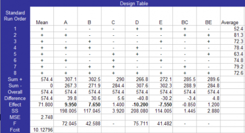
The calculations for this design table are given in the previous newsletters on experimental design techniques. Factors that account for less than 5% of the total sum of squares were considered to be insignificant. These were used to form the mean square error. F values were then calculated based on this mean square error. F values greater than the critical value of F were considered significant. Details of the calculations are given in the instruction manual accompanying the software.
The second part of the statistical analysis is the analysis of variance (ANOVA). ANOVA table (Table 4) reports the significance of each input variable and their interactions. The significant effect is determined based on the level of probability (p-value). Since this study was conducted by using one replicate per each factorial combination, the estimation of the error sum of squares (SSE) can not be performed. Therefore, the p-value of each factor can not be determined in this case. More information on the ANOVA table can be found in our last newsletter (click here).
Table 4: ANOVA Table
| Source of Variation | SS | df | MS | F | p value | % Cont |
| A | 198.005 | 1 | 198.005 | N/A | N/A | 30.68% |
| B |
117.045 | 1 | 117.045 | N/A | N/A | 18.14% |
| C |
3.92 | 1 | 3.92 | N/A | N/A | 0.61% |
| D |
208.08 | 1 | 208.08 | N/A | N/A | 32.24% |
| E | 114.005 | 1 | 114.005 | N/A | N/A | 17.66% |
| BC | 1.445 | 1 | 1.445 | N/A | N/A | 0.22% |
| BE |
2.88 | 1 | 2.88 | N/A | N/A | 0.45% |
| Error | 0 | 0 | ||||
| Total | 645.38 | 7 |
Even though the p-value is not available, you can use the % contribution column to determine which variables may have a significant impact on the yield. You can see that A, B, D, and E appear to be significant. This agrees with the results from the design table.
The SPC for MS Excel software allows you to delete the insignificant effects and rerun the analysis. A new ANOVA was run without factor C and the two interactions. This new ANOVA is shown in Table 5.
Table 5: Revised ANOVA Table
| Source | SS | df | MS | F | p value | % Cont |
| A | 198.005 | 1 | 198.005 | 72.045 | 0.0034 | 30.68% |
| B | 117.045 | 1 | 117.045 | 42.588 | 0.0073 | 18.14% |
| D | 208.080 | 1 | 208.080 | 75.711 | 0.0032 | 32.24% |
| E | 114.005 | 1 | 114.005 | 41.482 | 0.0076 | 17.66% |
| Error | 8.245 | 3 | 2.748333 | |||
| Total | 645.380 | 7 |
The removal of the interactions from the linear model allows the error term to have 3 degrees of freedom and the calculation of mean square error (MSE). Consequently, the F test of each input variable can be calculated by dividing the MS of a factor by the MS of the error. The significant effects are those with p-value less that or equal to 0.05. All factors are significant.
Table 6 is the model’s ANOVA. It reports the significance of the selected model in explaining the total variability in % yield. The model p-value “0.0036′ clearly demonstrates that the model is significant. This implies that the linear model is capable of explaining the total variation in % yield.
Table 6: Model ANOVA
| Source | SS | df | MS | F | p value |
| Model | 637.135 | 4 | 159.284 | 57.956 | 0.0036 |
The software generates other statistics including the R Square value and the R Square Prediction value.
- R Square: 98.72%
- R Square Prediction: 90.92%
R Square is the measure of the model contribution to the total variation in the % yield. The R Square value 98.72% suggests that almost 100% of the variability in % yield can be explained by the four input variables. The R Square Prediction value measures the model predictive capability with a new set of raw data. The R Square Prediction value is 90.92%.
The software also provides the regression coefficients for both the coded and original (uncoded) factor levels. These are shown in Table 7.
Table 7: Regression Coefficients
| Coded | UnCoded | |||||
| Y= | 71.800 | Intercept | Y= | 49.325 | Intercept | |
| + | 4.975 | A | + | 19.900 | % B | |
| + | 3.825 | B | + | 0.765 | % GW | |
| + | -5.100 | D | + | -0.026 | SS | |
| + | -3.775 | E | + | -1.887 | ST |
The coded equation gives you the most information because you can judge the relative impact of the factors. Factor D has a coefficient of -5.1. The absolute value of this coefficient is the largest of the four. Thus, it has the largest impact. The equation based on the coded factors is then:
Yield = 71.8 + 4.975A + 3.825B – 5.1D – 3.775E
Step 6: Develop Conclusions
The results indicate that speed and length of the spheronizer (SS and ST) process within the studied range had negative effect on the yield of desired quality pellets while the % binder and % granulation water showed positive effect on the yield of proper pellets quality. The negative effects of SS and ST can be understood by the fact that high SS and/or long ST cause the pellets to stick together making triplicates and quadruplicates, which itself makes the pellets to grow larger than the desired sizes.
Granulation time (GT) in this study was selected based on prior experience with the extrusion – spheronization process. It seems that the selected GT range had very small effect on the yield by not affecting the texture and consistence of granulated powder.
This study has determined which of the five factors had a significant impact on the yield. Confirmation runs would be required to ensure that the results are valid. For example, if the objective was to maximize the yield, the % binder and % granulation water would be set to their high levels while the speed and length of the spheronizer would be set to their low levels. The predicted yield is:
Yield = 71.8 + 4.975(1) + 3.825(1) – 5.1(-1) – 3.775(-1) = 89.475%
References
- John Peterson. What your ICH Q8 design space need: A Multivariate Predictive Distribution, GlaxoSmithKline Pharmaceuticals.
- ICH Q 8 (R2), Pharmaceutical Development, Step 4 Version, Aug. 2009.
- Erkoboni, D.F., “Extrusion-Spheronization as a Granulation Technique” in Handbook of Pharmaceutical Granulation Technology, Edited by Dilip M. Parikh (Marcel Dekker, Inc., NY), PP. 333-368.
Guest Author
This month’s newsletter is written by Nabil B. Darwazeh, Ph.D. Dr. Darwazeh is currently a Research and Development Technical Advisor and Process Scale-Up Manager at United Pharmaceutical, Amman, Jordan. Before Joining United Pharmaceutical, he was Senior Research Scientist at Wyeth Pharmaceuticals, Pearl River, NY, and Research Scientist at Mallinckrodt Veterinary, Mundelein, IL.
He received his Bachelor’s Degree in Agriculture Sciences from University of Baghdad in 1980, and his Master’s Degree in Animal Science from California State University in 1983. Dr. Darwazeh received the Ph.D. Degree in Medicinal Chemistry and Pharmaceutical Sciences from University of Kentucky in 1995. Dr. Darwazeh is a member of the International Society for Pharmaceutical Engineering (ISPE).