In This Issue:
- Comparing Multiple Treatments
- Bonferroni’s Method
- Confidence Intervals
- Conclusion
- Summary
- Quick Links
Best wishes to all of you in this New Year. This marks the start of our sixth year of newsletters. This month’s newsletter will examine one method of comparing multiple process means (treatments). The method we will use is called Bonferroni’s method. We will build on the analysis we started last month using ANOVA.
Comparing Multiple Treatments
Quite often, you will want to test a single factor at various treatments. For example, you might want to test the yield of four different wheat varieties. The single factor is wheat and there are four different treatments (varieties). We will continue with the example we used last month.
The example is from the excellent book Design and Analysis of Experiments, 6th Edition, by Douglas C. Montgomery. The example involves a plasma etching process. An engineer wants to determine if there is a relationship between the power setting and the etch rate. She is using four different power settings (160W, 180W, 200W and 220W). The engineer tested five wafers at each power level. The data from the experiment are shown below.
| Treat/Power | 160 | 180 | 200 | 220 |
| 1 | 575 | 565 | 600 | 725 |
| 2 | 542 | 593 | 651 | 700 |
| 3 | 530 | 590 | 610 | 715 |
| 4 | 539 | 579 | 637 | 685 |
| 5 | 570 | 610 | 629 | 710 |
| Mean | 551.2 | 587.4 | 625.4 | 707.0 |
| St. Dev. | 20.017 | 16.742 | 20.526 | 15.24 |
The experiments were run in random order. The four power settings are the column headings. The results for each of the five wafers from each setting are below the headings. For example, when the power setting was 160, the five etch rates obtained were 575, 542, 530, 539 and 570.
The table above shows the means for each treatment. The means are not equal. Of course, this is not unexpected. Normal process variation will cause means to be different. The first question we want to answer is:
“Are there any significant differences in the treatment means?”
Last month we used Analysis of Variance (ANOVA) to answer this question. ANOVA was testing the following two hypotheses:
Ho: μ1= μ2= μ3= μ4
H1: μi ≠ μj for at least one i and one j
where μ is a treatment mean. The F test was used to determine which hypothesis was accepted. As shown last month, the null hypothesis (Ho) was rejected. This implies that there are significant differences between at least two of the four means. But this does not tell you which means are different. We will use Bonferroni’s method to determine this.
Bonferroni’s Method
This method answers the question:
“Which treatment means are significantly different from each other?”
Bonferroni’s method provides a pairwise comparison of the means. To determine which means are significantly different, we must compare all pairs. There are k = (a) (a-1)/2 possible pairs where a = the number of treatments. In this example, a= 4, so there are 4(4-1)/2 = 6 pairwise differences to consider.
To start, we must select a value for alpha (α), the confidence level. We will select α = 0.05. In Bonferroni’s method, the idea is to divide this family wise error rate (0.05) among the k tests. So each test is done at the α/k level.
We will use the t distribution to help determine the pairwise confidence interval. To start, we need to calculate the pooled variance. This is an estimate of the variance based on the four treatment means. The following equation is used to determine the pooled variance:
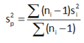
where ni is the sample size and si is the standard deviation for the ith sample. The standard deviations are given in the table above. The pooled variance for this data is then:
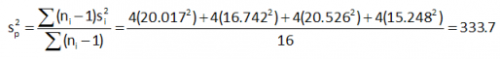
If you look at the ANOVA table from last month, you will see that this value corresponds to the mean square error.
The Bonferroni method says a pairwise difference is significant if:
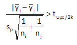
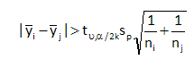
The right-hand side of this equation is the critical value. Any difference in pair of means that is larger than this will be significant.
The first step is to determine the value of t. Many statistical books contain tables of the t distribution. You can also determine t using the TINV function in Excel. The degrees of freedom used for t is the degrees of freedom associated with the pooled variance. In this case, there are 16 degrees of freedom (4 for each treatment). The value of α/2k is 0.00833. Using the t distribution table or the TINV function in Excel, the value of t is 3.008317. (Note: if you use TINV, the value of α you enter is α/2 to return the one-tail t value).
The pooled standard deviation is simply the square root of the pooled variance. Thus, sp = 18.26746.
The critical value is then:
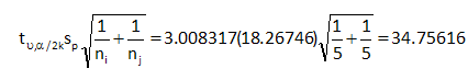
This number is then compared to the difference in means for each possible combination of treatment means. These differences are shown below.
| Comparisons | Difference in Means |
| 160W – 180W | 36.2 |
| 160W – 200W | 74.2 |
| 160W – 220W | 155.8 |
| 180W – 200W | 38 |
| 180W – 220W | 119.6 |
| 200W – 220W | 81.6 |
The table above shows that each difference is larger than the critical value. This means that there are significant differences between all treatment means.
Confidence Intervals
Part of the output from the SPC for Excel program using Bonferroni’s method to analyze this data is shown below. This table includes the confidence intervals for each difference in means. These are determined simply by adding and subtracting the critical value from the difference in the treatment means. As long as the confidence interval does not contain 0, there is significant difference in the two means.
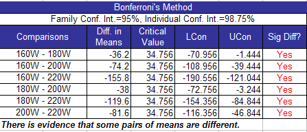
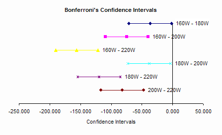
The confidence intervals can also be plotted as shown below. This shows that none of the intervals includes 0. All the treatment means are significantly different from one another.
Conclusion
This analysis has shown that there are significant difference between all treatment means. The ANOVA analysis last month showed that there was a significant difference between at least two of the means. The analysis this month shows that all treatment means are different. Bonferroni’s method is one way of doing this. This method spreads the value of α evenly across all pairs of treatment means. You should consider using this methodology to help you determine if there are significant differences in treatment means.
Summary
This month’s newsletter demonstrated how Bonferroni’s method can be used to compare multiple means. It answers the question which pair of means are significantly different from each other. The family wise error rate is divided equally over the paired averages. Confidence intervals are used to determine if there is a significant difference between the pair of means.