June 2023
 We often compare various treatments to see if there are any differences between the treatments. For example, we may want to compare how different types of fertilizers impact plant growth. Or how different catalysts impact reaction purity. We would like to find out the following:
Are there any differences in the means and, if so, which ones are significantly different?
You should also be concerned about differences in variation in the treatments, but we will only address the means here.
Analysis of Variance (ANOVA) is often used to determine if there is a difference between means. Unfortunately, ANOVA does not tell us which means are different from each other. Additional analysis is needed to do that. This is where pairwise comparisons of means comes in. This publication reviews how ANOVA lets us know that there are differences in the means and then examines three pairwise comparisons of means: Bonferroni method, Tukey method and Fisher’s least significant difference (LSD) method. Each methodology compares all pairs of means to determine if there are any significant differences.
Multiple pairwise comparisons do have an impact on the probability of deciding that at least one pairwise difference is significant when it is not. This is where the family error rate or family confidence interval comes in.
In this publication:
- Comparing Multiple Means
- ANOVA
- Pairwise Comparison of Means
- Fisher LSD Method
- Bonferroni Method
- Tukey Method
- Visual Picture of Pairwise Means Comparisons
- Summary
- Quick Links
Note that all the analysis done below was completed with the SPC for Excel software. Please feel free to leave a comment at the end of the publication. You may download a pdf copy of this publication at this link.
Comparing Multiple Means
The sample data used in this publication for pairwise comparisons of means comes from Statistics and Data Analysis by Ajit Tamhane and Dorothy Dunlop. There are six stations that create molded containers. The design weight of the container is 51.5 grams. An engineer is concerned that the weights at the stations are not uniform. The engineer selected 8 containers at random from each station and weighed the containers. The results are shown in Table 1.
Table 1: Plastic Container Weights (Grams)
| Station 1 | Station 2 | Station 3 | Station 4 | Station 5 | Station 6 | |
|---|---|---|---|---|---|---|
| 51.28 | 51.46 | 51.07 | 51.70 | 51.82 | 52.12 | |
| 51.63 | 51.15 | 51.44 | 51.69 | 51.70 | 52.29 | |
| 51.06 | 51.21 | 50.91 | 52.12 | 51.25 | 51.42 | |
| 51.66 | 51.07 | 51.11 | 51.23 | 51.68 | 51.88 | |
| 52.20 | 51.84 | 50.77 | 51.51 | 51.76 | 52.00 | |
| 51.27 | 51.46 | 51.86 | 52.02 | 51.63 | 51.84 | |
| 52.31 | 51.50 | 51.22 | 51.35 | 51.61 | 51.57 | |
| 51.87 | 50.99 | 51.54 | 51.36 | 52.14 | 51.74 | |
| Mean | 51.66 | 51.335 | 51.24 | 51.6225 | 51.69875 | 51.858 |
| Std. Dev. | 0.450 | 0.281 | 0.357 | 0.322 | 0.247 | 0.284 |
The sample mean and standard deviation for each station are shown. You can see that the sample means vary from a low of 51.24 and a high of 51.8575. It is not surprising that the sample means are different. Variation exists. There are differences in the sample means. But are there any sample means that are significantly different?
ANOVA
Analysis of variance is used to test the following null and alternate hypothesis:
H0: μ1= μ2= μ3 =……= μk
H1: μi ≠ μj for at least one i and one j
where μ is a treatment mean. The ANOVA table based on the data in Table 1 is shown below.
Table 2: ANOVA for Station Data
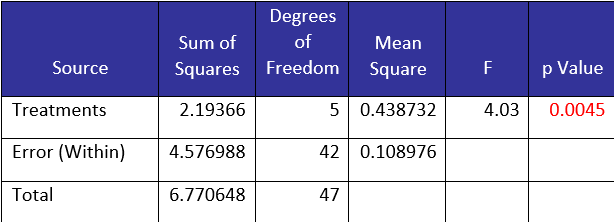
The first column in the ANOVA table contains the source of variation. It divides the sources of variation into two major categories: within treatment (error) and between treatment.
The objective is to determine if there are any differences between treatments (in this example, the stations). This is done by comparing the between treatments sum of square to the error sum of square. If the variance between treatments can be explained by the within treatment variance, we will conclude that there are no differences between the treatments. If the variance between treatments cannot be explained by the within treatment variance, we will conclude that there are differences between the treatments.
The second column in the table contains the sum of squares. These are calculated variances. For more information on ANOVA and the calculations, please see our SPC Knowledge Base article on Single Factor ANOVA.
The third column is the degrees of freedom. If “a” is the number of stations, the degrees of freedom for “between treatments” is a – 1. If N = the total number of observations, then the total degrees of freedom is N – 1 and the error degrees of freedom of N – a.
The fourth column is the mean square. The mean square is obtained by dividing the sum of squares for the source by the degrees of freedom for the source. Thus, MSE = SSError/(N-a). MSE is an estimate of the within treatment variation.
The fifth column is the F value. This is determined by dividing the mean square for the treatments by the mean square error. It is this value that determines if there are any significant differences between the treatment means.
The sixth column is the p-value. The p-value is the probability of getting that F value if the null hypothesis is true. If the p-value is small, we assume that it is not likely to get that F value if the null hypothesis is true and we conclude that there are differences in the means. p-values less than 0.05 are considered small.
In this example, p-value= 0.0045, which is small. So, we conclude that there are probably differences in the means of the six stations. But which stations are different? We will look at three methods to define which stations are different.
Pairwise Comparison of Means
There are several methods to compare means pairwise. In this publication, we will look at three: Fisher’s LSD method, the Tukey method, and the Bonferroni method. In each method, a critical value will be calculated. If the difference between two means is greater than the critical value, we will assume that those two means are significantly different – at least statistically.
The standard deviation (s) is used in the calculations below. This is the square root of the MSE. So,
s = 0.330
The t-distribution is also used in the calculations below. The degrees of freedom for the t value are the degrees of freedom based on the MSE. This is 42 as shown in the ANOVA table above.
Each method compares all possible pairs of means. There are k = (a) (a-1)/2 possible pairs where a = the number of treatments. Since there are 6 stations, then there are 6(6 – 1)/2 = 15 pairs of means to check.
Each pair of means is tested to the null hypothesis that μi = μj. We will start with Fisher’s LSD method.
Fisher’s LSD Method
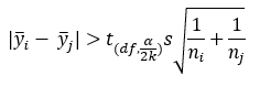
Fisher’s method compares each pair of means at the level , which is normally taken to be 0.05. The null hypothesis is rejected if the following is true for any pair of means:
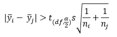
where the y terms represent the means of stations i and j, t is the t-value for the upper /2 percentile of the t distribution with df (degrees of freedom), s is the standard deviation, and the n terms represent the samples in the ith and jth stations.
The term to the right is sometimes referred as to the least significant difference (LSD).
For example, let’s compare the first and second station means, 51.66 and 51.335, respectively. The t value for 42 degrees of freedom and α = 0.05 is 2.018. The calculations can now be done.
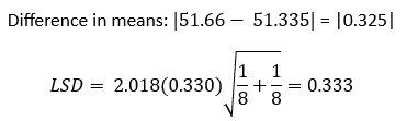
Since the range in the two means is less than the LSD value of 0.333, we conclude that the means for station 1 and station 2 are statistically the same. Table 3 shows the results for all 15 pairwise comparisons.
Table 3: Fisher LSD Method Results for Stations
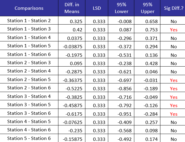
The table contains the pairwise difference means, the LSD value, the lower and upper 95% confidence intervals and whether there is a significant difference between the two pairs. The lower and upper 95% confidence intervals are obtained by subtracting and adding the LSD to the difference in means. The difference in pairs is statistically significant if the difference in means is greater than LSD or the confidence interval does not contain 0. There are six pairs which are statistically different:
- Station 1 – Station 3
- Station 2 – Station 5
- Station 2 – Station 6
- Station 3 – Station 4
- Station 3 – Station 5
- Station 3 – Station 6
Note that each pairwise test above was done with = 0.05, giving 95% confidence limits for each pairwise comparison. The problem is that we are making several comparisons. We have to worry about something called the Family Error Rate. The family error rate is the probability of coming to at least one false conclusion in a series of hypothesis tests. We will not go into the calculations here, but the family error rate for Fisher’s LSD method is 0.35. This gives a family confidence interval of 1 – 0.35 or 65%. This implies that there is a very good chance that there will be false conclusions in our results. It is because of this that Fisher’s LSD method is not used very often. The SPC for Excel software shows the results as follows:
Fisher Least Significant Difference (LSD) Method: Family Conf. Int.=65.03%, Individual Conf. Int.=95%
Bonferroni Method
The Bonferroni method controls the family error rate by dividing the desired family error rate (e.g., 0.05) among the k pairwise comparisons. In our example, there are 15 pairwise tests. So, the individual error rate becomes 0.05/15 = 0.003333.
Now the null hypothesis for means i and j is rejected if the following is true:
Note that the only difference between this and Fisher’s LSD method is the presence of 2k in the t value instead of just 2. This changes the t value. In this example, with 42 degrees of freedom and dividing α by 2k, the value of t is 3.112. The critical value for the Bonferroni method is the term on the right.
Consider stations 1 and 2 again. The critical value is given by:
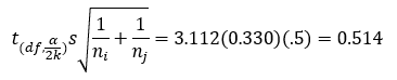
The difference in means for stations 1 and 2 is 0.325. The Bonferroni method shows that there is not a significant difference between the means for stations 1 and 2. Table 4 shows the results for all 15 pairwise comparisons for the Bonferroni method.
Table 4: Bonferroni Method Results for Stations
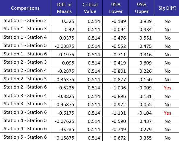
The columns are the same as for Fisher’s LSD method. Note that, however, with the Bonferroni method, only two pair of means are significantly different:
- Station 2 – Station 6
- Station 3 – Station 6
The difference is because the way the Bonferroni method controls the family rate:
Bonferroni’s Method: Family Conf. Int.=95%, Individual Conf. Int.=99.67%
The family confidence interval is 95% compared to 65% for Fisher’s LSD method. There are less false signals with the Bonferroni method.
Tukey Method
The Tukey method, like the Bonferroni method, tests at the family confidence interval – again usually 95% when α = .05. However, the Tukey method is a little more difficult because it uses the Studentized range distribution. The Studentized range (q) is the difference between the largest and smallest data point in a sample, measured in terms of sample standard deviations. It depends on the number of means (a), the degrees of freedom (df), and alpha.
With the Tukey Method, the null hypothesis for means i and j is rejected if:
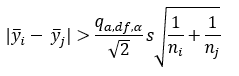
For 6 means, 42 degrees of freedom and α = 0.05, the value of the Studentized range distribution (q) is 4.2233. The values of the Studentized range distribution are available in tables in statistical books. Most software calculates the values. Again, the critical value is the term on the right side of the equation above.
For stations 1 and 2, the critical value is given as:
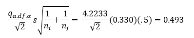
The difference in means for stations 1 and 2 is 0.325. The Tukey method shows that there is not a significant difference between the means for stations 1 and 2. Table 5 shows the results for all 15 pairwise comparisons with the Tukey Method
Table 5: Tukey Method Results for Stations
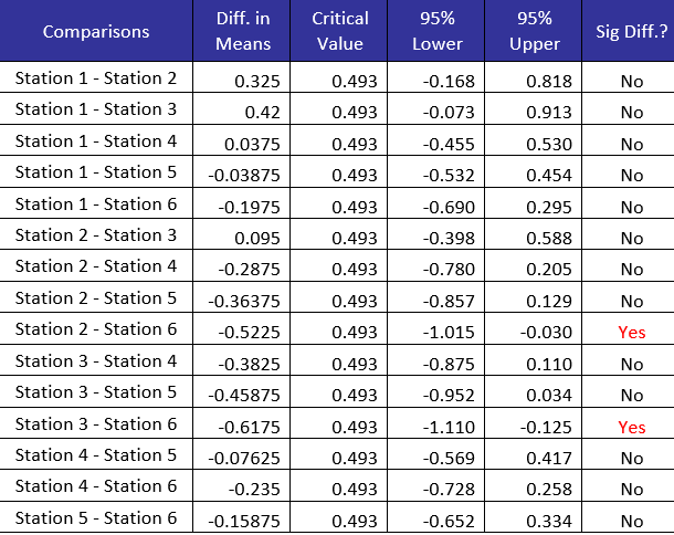
The Tukey method shows that two pairs have significant differences in means. The two are:
Station 2 – Station 6
Station 3 – Station 6
This is the same as Bonferroni’s method found. The family and individual confidence intervals for the Tukey method are shown below:
Tukey’s Test: Family Conf. Int.=95%, Individual Conf. Int:=99.53%, q(a,f,p)=4.2233
Visual Picture of Pairwise Means Comparisons
The tables above indicate which pairs have significantly different means. Sometimes it is best to look at results in charts if at all possible. You can do this by plotting the confidence intervals. Figure 1 shows the plot for the Tukey method.
Figure 1: Tukey Method 95% Confidence Intervals
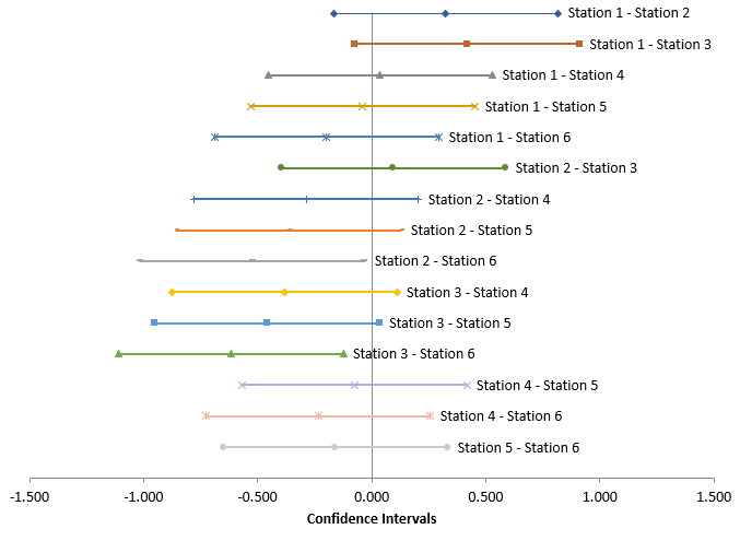
If an interval does not contain 0, then there is significant difference in the two means. This is true for Station 2 – Station 6 and Station 3 – Station 6.
Summary
This publication has examined three pairwise methods to determine which means are different when ANOVA indicates that there are significant differences in the means. For each method, a critical value is determined. If the range between a pair of means is greater than the critical value, then there is a significant difference between those two means.
Fisher’s LSD method controls the individual confidence interval but does not control the family confidence interval. For this reason, it is not preferred. Both the Bonferroni method and the Tukey method control the family confidence interval. These are preferred over Fisher’s LSD method.
You can get a visual picture of the results by plotting the confidence intervals for each pair. If the interval does not contain 0, then there is a significant difference in the means.