August 2020
(Note: all the previous SPC Knowledge Base in the process capability category are listed on the right-hand side. Select this link for information on the SPC for Excel software. SPC for Excel does perform Poisson Capability Analysis.)

The Poisson distribution is the probability model that is used when you are counting defects. This month’s publication examines how process capability works with the Poisson distribution. In addition to determining the capability, you must address the three key issues of stability, having enough data, and ensuring that the data follows a Poisson distribution.
In this issue:
- Counting Type Data
- Assumptions to Use the Poisson Distribution
- Poisson Process Capability Example Data
- Definition of the Poisson Process Capability
- The Issue of Stability: The u Control Chart
- The Issue of Enough Data: The Cumulative Defects per Unit Chart
- The Issue of Following a Poisson Distribution
- Defects per Unit vs Subgroup Size Chart
- P-P Plot
- Histogram
- Summary
- Quick Links
Please feel free to leave a comment at the end of the publication. Also, you may download a pdf copy of this publication at this link.
Counting Type Data

You can monitor the number of blemishes over time by counting the number of bubbles on an area of the plastic film. That area is the area of opportunity for defects to occur. The number of blemishes is called the number of defects.
A defect occurs when something does not meet a preset specification. Again, it does not mean that the item itself is defective. When looking at counting data, you have whole numbers such as 0, 1, 2, 3; you cannot have half of a defect. With the plastic film example, you will have 1 blemish, 2 blemishes, etc.
Under certain conditions, the number of defects follows a Poisson distribution. This distribution is used to model the number of occurrences of a defect when the number of opportunities is large, but the actual number of defects that occur is small.
Assumptions to Use the Distribution
There are four conditions that must be met to use the Poisson distribution. These are listed in Advanced Topics in Statistical Process Control (Dr. Wheeler, www.spcpress.com) as follows:
- The counts must be discrete counts (e.g., each blemish that occurs is discrete).
- The counts must occur in a well-defined region of space or time (e.g., one plastic film is the well-defined region of space where the blemishes can occur).
- The counts are independent of each other, and the likelihood of a count is proportional to the size of the area of opportunity (e.g., the probability of finding a blemish on a plastic film is not related to which part of the plastic film is selected).
- The counts are rare compared to the opportunity (e.g., the opportunity for blemishes to occur in the plastic film is large, but the actual number that occurs is small).
If these conditions are met, then the Poisson distribution can be used to model the process.
Poisson Process Capability Example Data
We will continue with the blemishes in the plastic film process to explore the Poisson Process Capability. Data are collected once an hour on the plastic film. An area is cut out and the blemishes are counted. The area in cm2 and the number of blemishes are recorded. The data for the last 50 hours are shown in Table 1.
Table 1: Blemishes Data
| Hour | Blemishes | Area | Hour | Blemishes | Area | |
|---|---|---|---|---|---|---|
| 1 | 3 | 8 | 26 | 4 | 12 | |
| 2 | 2 | 9 | 27 | 3 | 9 | |
| 3 | 4 | 8 | 28 | 5 | 12 | |
| 4 | 6 | 9 | 29 | 4 | 10 | |
| 5 | 2 | 12 | 30 | 2 | 10 | |
| 6 | 4 | 10 | 31 | 1 | 11 | |
| 7 | 1 | 10 | 32 | 1 | 8 | |
| 8 | 3 | 8 | 33 | 5 | 12 | |
| 9 | 6 | 11 | 34 | 6 | 10 | |
| 10 | 3 | 11 | 35 | 2 | 12 | |
| 11 | 1 | 12 | 36 | 1 | 8 | |
| 12 | 6 | 10 | 37 | 5 | 9 | |
| 13 | 1 | 9 | 38 | 4 | 10 | |
| 14 | 4 | 9 | 39 | 4 | 8 | |
| 15 | 1 | 11 | 40 | 4 | 12 | |
| 16 | 3 | 12 | 41 | 2 | 10 | |
| 17 | 0 | 12 | 42 | 1 | 9 | |
| 18 | 4 | 12 | 43 | 2 | 12 | |
| 19 | 1 | 11 | 44 | 1 | 8 | |
| 20 | 2 | 11 | 45 | 4 | 10 | |
| 21 | 3 | 12 | 46 | 2 | 11 | |
| 22 | 2 | 12 | 47 | 2 | 12 | |
| 23 | 5 | 9 | 48 | 5 | 9 | |
| 24 | 2 | 11 | 49 | 4 | 8 | |
| 25 | 4 | 9 | 50 | 2 | 12 |
The specification for the plastic film is 0.8 or less blemishes per cm2 area. We will use the Poisson Process Capability technique to answer the question of how capable the process is.
Definition of the Poisson Process Capability
Last month we examined the Binomial Process Capability technique. This is used when you have yes/no type data. The steps in the Poisson Process Capability technique are essentially the same as those in the Binomial Process Capability – the difference being that we are using the Poisson distribution instead of the binomial. But the steps in the process – and the questions being answered below – are very much the same.
The definition of the Poisson Process Capability is simple. It is the average defects per unit (DPU) over time. Straightforward and simple. Well, almost.
To get the average DPU, you total the number of blemishes (149) and divide that number by the total area examined (512). With the Poisson data, c is the number of blemishes and n is the sample size (area). The average is given by u.
u= (∑c)/(∑n)=149/512=0.291
The process capability of the plastic film process is 0.291 defects per unit (where the unit is 1 cm2). This is the capability of the process. 0.291 DPU is what the process is capable of producing on average. The question you now must answer is
“Is this a good average for the process?”
So, a better definition of Poisson Process Capability is the average defects per unit over time that is valid. To be a valid average, the answer to the following three questions must be yes:
- Is the process in statistical control?
- Are there enough data?
- Does the data follow the Poisson distribution?
Below we show how to answer these questions.
The Issue of Stability: The u Control Chart
The first step in determining if the average is valid is to check the stability of the process using a control chart. The u control chart is used for this. The u value for each sample is plotted on the control chart. The value is given by c/n for each sample.
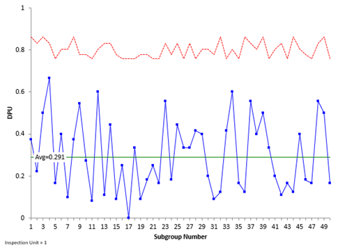
The average and control limits (based on the Poisson distribution) are then calculated and plotted on the u control chart. If there are no points beyond the control limits or patterns, the process is said to be in statistical control. If a process is in statistical control, there are only common causes of variation present and no special causes present. Figure 1 is the u control chart for the number of blemishes. The dotted line is the upper control limit.
Figure 1: u Control Chart for Blemishes
There are no points beyond the control limits and no patterns in the data. The process is in statistical control.
Please see our SPC Knowledge Base article Attribute Control Charts Overview for more information on u control charts. You can also see our SPC Knowledge Base article When an Average Isn’t the Average for more information on how the state of control of a process impacts the average.
The Issue of Enough Data: The Cumulative Defects per Unit Chart
Your control chart needs to have enough data to be sure that the average is valid. For example, you may have an in-control process after five data points. Would you be comfortable that these five data points would give you a valid average for the process? They might, but probably they are going to be off from the true average. The cumulative DPU chart addresses this issue.
The cumulative DPU chart plots the cumulative average DPU over time. For example, after the first five points, the total number of blemishes was 17 and the total area inspected was 46. The cumulative average DPU after those first five points is:
u= (∑c)/(∑n)=17/46=0.370
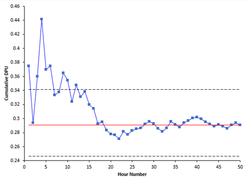
After five points, the cumulative average DPU is 0.370 compared with 0.291 for all the data. Five points is probably not enough. Figure 2 is the plot for the cumulative average DPU over time.
Figure 2: Cumulative DPU Chart
Figure 2 is used to determine if you have enough samples for a valid estimate of the average DPU. The center line is the average DPU ( u, the same as the center line on the u control chart). The upper and lower confidence limits for the average DPU are also plotted. We will not deal with those here as they are not necessary to interpret this chart.
You want the cumulative DPU average to flatten out along u. It should cross the centerline several times as it flattens out. If this occurs, you have enough samples. This does occur in this example, so you have enough data. The answer to the second question above is yes.
The Issue of Following a Poisson Distribution
At this point, there are enough data for an in-control process to have a valid average – if the data follows a Poisson distribution. There are three charts that can be used to help decide if the data follows a Poisson distribution: one is the DPU per sample versus the sample size chart if the sample size varies; another is the P-P plot if the sample size remains the same. Both are described below along with the histogram of the sample DPU values.
DPU vs Sample Size Chart
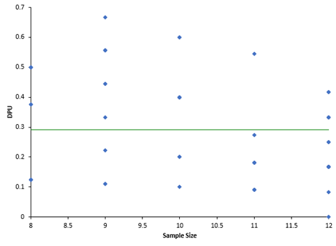
This chart plots the DPU for each sample versus the sample size. The chart is shown in Figure 3.
Figure 3: DPU vs Sample Size Chart
If the data are from a Poisson distribution, you would expect the points to be randomly distributed around the centerline, which is the average DPU (u = 0.291). The average (u) is used in all three charts so far. You can see from Figure 3, the points appear to be randomly distributed around the centerline, so it appears the data comes from a Poisson distribution.
P-P Plot
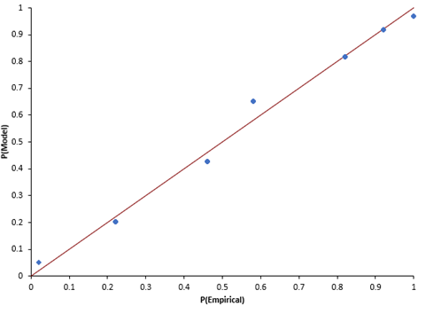
If the sample size is constant, you cannot make a plot like Figure 3. Instead, you can make a P-P Plot to determine if the data comes from a Poisson distribution. The P-P Plot shows the empirical cumulative distribution function (CDF) values (based on the data) against the theoretical CDF values (based on the Poisson distribution). If the P-P Plot is close to a straight line, then the Poisson distribution fits the data. Figure 4 is an example of the P-P plot for the data above with a constant sample size.
Figure 4: P-P Plot
The points fall about the straight line so you can assume that the data comes from a Poisson distribution.
Histogram
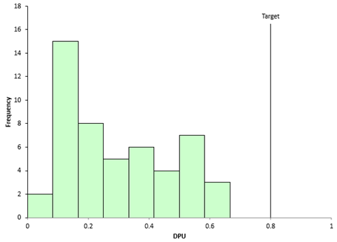
The histogram can be used to see what the distribution of DPU values looks like as shown in Figure 5.
Figure 5: DPU Histogram
Does this look like a Poisson distribution? It is hard to tell sometimes when looking at DPU. But it does show you the distribution of values and the relationship of the DPU values to the target or specification. All samples have met the target – and since the process is in statistical control, it should continue to meet the target into the future.
Summary
This publication examined Poisson Process Capability. This is the average defects per unit as long as the four criteria for using a Poisson distribution are satisfied and the answers to the following three questions are yes:
- Is the process in statistical control?
- Are there enough data?
- Do the data follow the Poisson distribution?
The u control chart is used to determine if the process is in statistical control, while the cumulative DPU chart is used to determine if there are sufficient data. Finally, the DPU versus sample size chart, the P-P plot, or the histogram can be used to determine if the data comes from a Poisson distribution.
Very Good article.Am I wrong if I find the Sigma level based on DPU obtained as in the article and using normal distribution tabel (6 sigma ST and 4.5 sigma LT for 3.4 DPMO?
The data in this article are Poisson, not normal distribution. So you can't use a normal distribution table.