July 2020
(Note: all the previous SPC Knowledge Base in the process capability category are listed on the right-hand side. Select this link for information on the SPC for Excel software. SPC for Excel does perform Binomial Capability Analysis.)
When someone mentions process capability, we usually think about Cpk and Ppk. These are process capability metrics for determining if the process is capable of meeting customer expectations. Our SPC Knowledge Base contains multiple articles on process capability for both normal and non-normal distributions. These articles are for continuous distributions, and the process capability techniques compare those distributions to the customer specifications.

For example, there were 50 telemarketing calls one day and 2 of those resulted in an order. The % of telemarketing calls resulting in an order for that day is 2/50 = 4%. What is your telemarketing process capable of producing?
The binomial distribution is the probability model that is used when there are two possible outcomes. This month’s publication examines how process capability works with this binomial distribution. It is really quite simple as you will see. In this issue:
- Yes/No Type Data
- Assumptions to Use the Binomial Distribution
- Binomial Process Capability Example Data
- Definition of the Binomial Process Capability
- The Issue of Stability: The p Control Chart
- The Issue of Enough Data: The Cumulative % Defectives Chart
- The Issue of Following a Binomial Distribution
- % Defectives vs Subgroup Size Chart
- P-P Plot
- Histogram
- Summary
- Quick Links
You may download a pdf version of this publication at this link. Please feel free to leave a comment at the end of the publication. All the charts below were created using SPC for Excel’s Binomial Capability Analysis technique.
Yes/No Type Data
With yes/no type of data, you are examining a group of items. For each item, there are only two possible outcomes: either it passes, or it fails some preset specification. Each item inspected is either defective (i.e., it does not meet the specifications) or is not defective (i.e., it meets specifications). The example above used telemarketing calls. Other examples of yes/no data include:
- mail delivery: is it on time or not on time?
- phone answered: is it answered or not answered?
- invoice correct: is it correct or not correct?
- stock item: is it in stock or not in stock?
- cycle count: is it correct or not correct?
- product: is it in-spec or out of spec?
- supplier: material received on-time or not on-time?

Suppose one workshop has 20 attendees. This is the subgroup size (n). A “defective” participant is one who does not complete the requirements. The number of participants in the workshop who do not complete the requirements is denoted by np. Suppose that two participants do not complete the requirements, i.e., np = 2. The fraction defective is called p. In this example, p = np/n = 2/20 = .10 or 10% of the participants did not meet the requirements. As an instructor, you can track this data for each workshop.
Yes/no data are governed by the binomial distribution. The binomial distribution is used to obtain the probability of observing np successes (or failures) in n trials, with the probability of success on a single trial equal to p.
Assumptions to Use the Binomial Distribution
Yes/no data involves counts. You are counting items. To assume that the binomial distribution applies to the counts, the following four conditions must be satisfied (Advanced Topics in Statistical Process Control, Dr. Don Wheeler, www.spcpress.com):
- The area of opportunity for defective items to occur must consist of n distinct items (e.g., there are 20 distinct participants in the workshop)
- Each of the n distinct items is classified as possessing or not possessing some attribute (e.g., for each student, determine if the requirements were met or not met)
- Let p be the probability that an item has the attribute; p must be the same for all n items in a sample (e.g., the probability of a participant meeting or not meeting the requirements is the same for all participants).
- The likelihood of an item possessing the attribute is not affected by whether or not the previous item possessed the attribute (e.g., the probability that a participant meets or does not meet the requirements is not affected by others in the group).
If these four conditions are met, the binomial distribution can be used to estimate the distribution of the counts.
Binomial Process Capability Example Data
We will return to the telemarketing calls and use the data describing that situation. There is a team that does telemarketing calls daily. The number of calls each day is n, the subgroup size. The number of calls that result in an order is np, the number of “defectives.” The data for the last 50 days is given in Table 1.
Table 1: Telemarketing Calls Data
| Day | Calls Resulting in an Order (np) | Number of Calls (n) | Day | Calls Resulting in an Order (np) | Number of Calls (n) | |
|---|---|---|---|---|---|---|
| 1 | 1 | 48 | 26 | 3 | 48 | |
| 2 | 2 | 41 | 27 | 3 | 56 | |
| 3 | 2 | 42 | 28 | 3 | 48 | |
| 4 | 2 | 52 | 29 | 2 | 56 | |
| 5 | 2 | 42 | 30 | 2 | 53 | |
| 6 | 4 | 57 | 31 | 6 | 51 | |
| 7 | 0 | 60 | 32 | 2 | 55 | |
| 8 | 3 | 57 | 33 | 4 | 48 | |
| 9 | 4 | 43 | 34 | 1 | 47 | |
| 10 | 2 | 60 | 35 | 2 | 55 | |
| 11 | 1 | 54 | 36 | 5 | 44 | |
| 12 | 1 | 50 | 37 | 3 | 48 | |
| 13 | 2 | 40 | 38 | 2 | 44 | |
| 14 | 1 | 44 | 39 | 2 | 55 | |
| 15 | 6 | 52 | 40 | 1 | 48 | |
| 16 | 1 | 50 | 41 | 1 | 53 | |
| 17 | 2 | 60 | 42 | 0 | 46 | |
| 18 | 0 | 41 | 43 | 3 | 60 | |
| 19 | 2 | 45 | 44 | 2 | 52 | |
| 20 | 4 | 59 | 45 | 1 | 49 | |
| 21 | 4 | 44 | 46 | 1 | 47 | |
| 22 | 2 | 50 | 47 | 1 | 55 | |
| 23 | 2 | 53 | 48 | 2 | 47 | |
| 24 | 0 | 47 | 49 | 5 | 49 | |
| 25 | 2 | 50 | 50 | 2 | 59 |
We will assume that these data satisfy the criteria above to use the binomial distribution. We will use these data to create a Binomial Process Capability.
Definition of the Binomial Process Capability
The definition of the Binomial Process Capability is quite simple. It is the average percentage defective over time. That’s it! Pure and simple! It is what your process is capable of generating. Well, there is a little more to the definition.
To get the average percentage defective, you total the number of calls resulting in an order (111) and divide that number by the total number of calls (2514) and multiply by 100. The average is given by p.
p=(∑np)/(∑n)=111/2514=4.42%
The process capability of the telemarketing calls process is 4.42%. On average, 4.42% of the telemarketing calls result in an order. That is the capability of the process. The question you now must answer is:
“Is this a good average for the process?”
So, a better definition of Binomial Process Capability is the average percentage defective over time that is valid. To be a valid average, the answer to the following three questions must be yes:
- Is the process in statistical control?
- Are there enough data?
- Does the data follow the binomial distribution?
Let us look at some tools to help answer these three questions.
The Issue of Stability: The p Control Chart
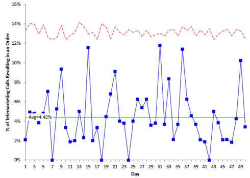
The first step in determining if the average is valid is to check the stability of the process using a control chart. The p control chart is used for this. The p value for each subgroup (p = np/n) is plotted on a p control chart. The average and control limits (based on the binomial distribution) are then calculated and plotted on the p control chart. If there are no points beyond the control limits or patterns, the process is said to be in statistical control. If a process is in statistical control, there are only common causes of variation present and no special causes present. Figure 1 is the p control chart for the telemarketing data. The dotted line is the upper control limit.
Figure 1: p Control Chart for Telemarketing Data
There are no out of control points in Figure 1. The process is stable – it is consistent and predictable. So, the average (4.42%) is valid. It was not calculated with the presence of special causes. It represents the average of the stable process. The answer to the first question above is yes – the process is in statistical control.
The control limits are not straight since the subgroup size varies (the calls per day). Please see our SPC Knowledge Base article Attribute Control Charts Overview for more information on p control charts. You can also see our SPC Knowledge Base Article When an Average Isn’t the Average for more information on how the state of control of a process impacts the average.
The Issue of Enough Data: The Cumulative % Defectives Chart
Your control chart needs to have enough data to be sure that the average is valid. For example, you may have an in-control process after five data points. Would you be comfortable that these five data points would give you a valid average for the process? They might, but probably they are going to be off from the true average. The cumulative % defective chart addresses this issue.
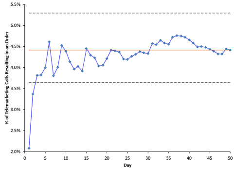
The cumulative % defectives chart plots the cumulative average over time. For example, after the first five points, the number of telemarketing calls resulting in an order was 9 out of a total of 225 calls. The cumulative average after those first five points is:
p=(∑np)/(∑n)=9/225=4.00%
After five points, the cumulative average is 4% compared with 4.42% for all the data. Five points is probably not enough. Figure 2 is the plot for the cumulative % defectives over time.
Figure 2: Cumulative % Defective Chart
Figure 2 is used to determine if you have enough subgroups (days) for a valid estimate of the average % defectives. The center line is the average % defective ( p, same as the center line on the p control chart). The upper and lower confidence limits for the average % defectives are also plotted. We will not deal with those here as they are not necessary to interpret this chart.
You want the cumulative % defectives value to flatten out along the average % defective line. It should cross the centerline several times as it flattens out. If this occurs, you have enough subgroups. This does occur in this example, so you have enough data. The answer to the second question above is yes.
The Issue of Following a Binomial Distribution
At this point, there are enough data for an in-control process to have a valid average – if the data follows a binomial distribution. After all, we used the p control chart, so we assumed we had a binomial distribution. There are three charts that can be used to help decide if the data follows a binomial distribution: one is the % defectives versus subgroup size chart if the subgroup size varies; another is the P-P plot if the subgroup size remains the same. Both are described below along with the histogram of the % defectives.
% Defectives vs Subgroup Size Chart
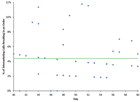
This chart plots the % defective for each subgroup versus the subgroup size. The chart is shown in Figure 3.
Figure 3: % Defective vs Subgroup Size Chart
If the data are from a binomial distribution, you would expect the points to be randomly distributed around the centerline, which is the average % defective (p ? = 4.42). The average (p) is used in all three charts so far. You can see from Figure 3, the points appear to be randomly distributed around the centerline, so it appears the data comes from a binomial distribution.
P-P Plot
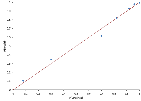
If the subgroup size is constant, you cannot make a plot like Figure 3. Instead, you can make a P-P Plot to determine if the data comes from a binomial distribution. The P-P Plot shows the empirical cumulative distribution function (CDF) values (based on the data) against the theoretical CDF values (based on the binomial distribution). If the P-P Plot is close to a straight line, then the binomial distribution fits the data. Figure 4 is an example of the P-P plot for the data above with a constant subgroup size of 50.
Figure 4: P-P Plot
The points fall along the straight line, so you assume the data came from a binomial distribution.
Histogram
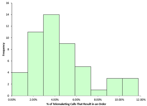
Of course, you can always do a histogram of the % defectives to see what the distribution looks like. Figure 5 is the histogram for the % of telemarketing calls that results in an order.
Figure 5: Histogram
Does this look like a binomial distribution? The binomial distribution changes shape based on the average and the sample size, so sometimes a histogram will not help you that much in determining if the data comes from a binomial distribution. But it does show you the distribution of values.
Summary
This publication examined Binomial Process Capability. This is the average % defective as long as the 4 criteria for using a binomial distribution are satisfied and the answers to the following three questions are yes:
- Is the process in statistical control?
- Are there enough data?
- Do the data follow the binomial distribution?
The p control chart is used to determine if the process is in statistical control, while the cumulative % defectives chart is used to determine if there are sufficient data. Finally, the % defectives versus subgroup size chart, the P-P plot, or the histogram can be used to determine if the data comes from a binomial distribution.
Great article. What happens when a process is required to attain a certain capability, that means, a claim for the p rate before data is available? How many sub-groups one would need to have?
Thanks. If it is a short run only, then you are stuck using the data you have with the caveats above; otherwise you want to have enough to the cumulative average has leveled off.