June 2008
In this Issue
This month is the first part of a series on linear regression. Linear regression is closely related to one of the basic SPC tools: the scatter diagram. A scatter diagram examines the relationship between two variables. It may be that one variable increases as the other increases or decreases. Our February 2005 publication explores scatter diagrams in more detail.
Linear regression can be used to mathematically define the relationship between two variables. We often want to know how the changes in one variable affect another variable. There is sometimes a straight line relationship between two variables. Linear regression helps us define this relationship. The major objective is to determine if one variable can be controlled by controlling another variable. Linear regression helps us build a model of the process. This is one method of decreasing process variation.
This month we will explore how the best fit linear equation is developed. Next month we will explore how to tell if the relationship is significant.
Regression Example
The following example demonstrates how linear regression works. This example is from the book Introduction to Linear Regression Analysis (Montgomery, Peck and Vinning, 4th edition, Wiley & Sons, 2006). This is an excellent book on regression for those of you who want to learn much more about regression.
The shear strength of the bond between two types of propellant is important in the manufacturing of a rocket motor. Someone asked the question, “Is the age of the propellant related to the shear strength?” To answer this question, twenty paired observations of shear strength and age of the propellant were collected. These are shown below.
| Observation | Shear Strength, Y (psi) | Age of Propellant, X (weeks) |
|---|---|---|
| 1 | 2158.7 | 15.5 |
| 2 | 1678.15 | 23.75 |
| 3 | 2316 | 8 |
| 4 | 2061.3 | 17 |
| 5 | 2207.5 | 5.5 |
| 6 | 1708.3 | 19 |
| 7 | 1784.7 | 24 |
| 8 | 2575 | 2.5 |
| 9 | 2357.9 | 7.5 |
| 10 | 2256.7 | 11 |
| 11 | 2165.2 | 13 |
| 12 | 2399.55 | 3.75 |
| 13 | 1779.8 | 25 |
| 14 | 2336.75 | 9.75 |
| 15 | 1765.3 | 22 |
| 16 | 2053.5 | 18 |
| 17 | 2414.4 | 6 |
| 18 | 2200.5 | 12.5 |
| 19 | 2654.2 | 2 |
| 20 | 1753.7 | 21.5 |
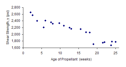
The scatter diagram for this data is shown below. As can be seen from the scatter diagram, there does appear to be a relationship. It appears that as the age of the propellant increases, the shear strength decreases. We can use regression analysis to quantify that relationship. This will also allow us to predict the shear strength based on the age of the propellant. We start by determining the best fit linear equation.
Method of Least Squares
In regression, y is the variable we want to predict (the dependent variable). In this example, y is the shear strength. x is the independent variable — in this case, the age of the propellant.
We begin by assuming that there is a linear relationship between the age of the propellant and shear strength. Remember, this does not mean there is a linear relationship. The methodology below will generate the best fit linear equation for almost any set of data. We must eventually decide if the model is useful to us. This relationship is described by the model below.
y = β0+β1x + e
where x is the propellant age and y is the shear strength. β0 and β1 are called parameters of the model. y consists of two parts:
- the value of β0+β1x
- e which is the error or the distance any value of y may fall off the regression line
The parameters in the model cannot be known exactly. However, we can make use of the data collected to estimate the parameters — just like we use process samples to estimate the average for control charts. If b0and b1are our estimates of β0 and β1, respectively, the model becomes:
yp= b0+ b1x
where yp is the predicted value of y for a given value of x once b0and b1have been determined. b1is the slope of the line. b0is the y-intercept (where the line crosses the y axis).
The method of least squares is used to determine the best fit line between x and y. Suppose, as in the data given in the table above, we have a series of observations for x and y. Suppose there are n sets of observations between x and y. We can denote these n sets as (x1, y1), (x2, y2), ……., (xn, yn). When we determine b0and b1, the model can be used to predict the values of y for given values of x. The difference between what the model predicts (yp) and what we actually get (yi) is called the residual (ei).
ei = yi – yp
The method of least squares is based on choosing b0 and b1 so that the sum of the squares of the deviations (residuals) is a minimum. If SSR is used to denote the sum of the squares of the deviations, we are trying to minimize the following:
SSR = S(yi – yp)2
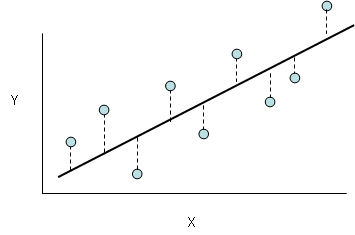
This is shown graphically in the figure below. A line fitted using the method of least squares minimizes the vertical dotted-line distances shown in the figure.
The next section shows how to calculate the best fit line for the example data.
Best Fit Equation
The best fit equation can be determined using the following equations:
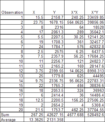
A variable with a bar over it means it is the average. The table below summarizes the calculations, which are normally done using software.
Using the data in the table, the following calculations can be done:
Sxx = 4677.6880*(267.25*267.25/20) = 1106.56
Sxy = 528,492.6 – (20)(13.3625)(2131.358)=-41,112.65
b1 = Sxy/Sxx = -41,112.65/1106.56 = -37.15
b0 =y – b1(x ) = 2131.358 – (-37.15)(13.3625) = 2627.82
Thus, the best fit equation for this data is:
y = 2627.82 + (-37.5)x
Conclusions
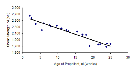
The best fit line has been added to the scatter diagram as shown below. The slope, b1, means that, on average, the shear rate decreases by 37.15 for each additional week of age of the propellant. Note that this model can be used to improve the process. For example, if the minimum shear strength is 2100, the age of the propellant can’t be more than 14 weeks.
A linear equation can always be fit to data. This does not mean that the regression is statistically significant or of any practical use. Next month’s newsletter will explore this issue.
Summary
Regression analysis was introduced this month. The objective of regression analysis is to see if there is a significant relationship between variables and to define that relationship using a best fit line. This involves calculating the slope (b1) and y-intercept (b0). The calculations were introduced. Next month we will look at how to determine if the “best fit” is of any use to you.


