In this issue:
Have you ever had to explain to anyone what a standard deviation is? Or perhaps, you aren’t sure yourself what it is. What is it used for? Why is it important in process improvement? When using control charts, the standard deviation, as well as the average, is a very important parameter. One must understand what is meant by the standard deviation. This newsletter addresses this. We will start with describing what an average is.
Average
The average (also called the mean) is probably well understood by most. It represents a “typical” value. For example, the average temperature for the day based on the past is often given on weather reports. It represents a typical temperature for the time of year.
The average is calculated by adding up the results you have and dividing by the number of results. For example, suppose we have wire cable that is cut to different lengths for a customer. These lengths, in feet, are 5, 6, 2, 3, and 8. The average is determined by adding up these five numbers and dividing by 5. In this case, the average (X) is:
X = (5+6+2+3+8)/5 = 4.8
The average length of wire for these five pieces is 4.8 feet.
Standard Deviation
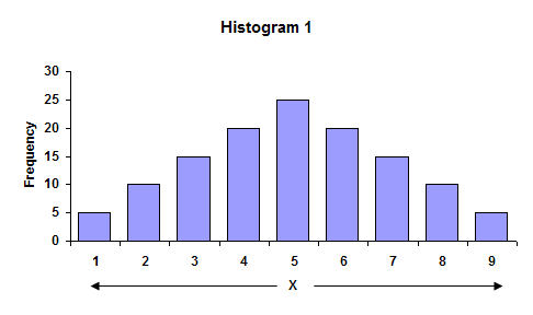
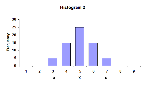
While the average is understood by most, the standard deviation is understood by few. To begin to understand what a standard deviation is, consider the two histograms. Histogram 1 has more variation than Histogram 2.
In the first histogram, the largest value is 9, while the smallest value is 1. The overall range of data is 9 – 1 = 8. In the second histogram, the overall range is 7 – 3 = 4. The range is larger for Histogram 1. Ranges are often used in control charts for variation (for example, the X-R charts). In fact, the average range from a control chart can be used to calculate the process standard deviation.
The average of the data in each histogram is 5. So, in this case, the highest bar is the average. We can also see that Histogram 1 has more variation than Histogram 2 because the distance, on average, of the individual observations from the overall average (5) is greater in Histogram 1 than Histogram 2. This distance is usually referred to as a deviation. If your have a result X = 3, the deviation of this value from the average is 3 – 5 = – 2 or the value “3” is two units below the average.
One can view the standard deviation as being an “average” distance each individual measurement is from the average, X. Let’s return to the numbers we found the average for earlier to see how we can estimate this average deviation from X. These numbers were the length of wire cable we had cut. We want to find the average distance each number is from X = 4.8. To do this, we can determine the deviation of each number from the average as shown below.
| Length (X) | Deviation from Average (X- X) |
| 5 | 5 – 4.8 = 0.2 |
| 6 | 6 – 4.8 = 1.2 |
| 2 | 2 – 4.8 = -2.8 |
| 3 | 3 – 4.8 = -1.8 |
| 8 | 8 – 4.8 = 3.2 |
If we add up the deviations from average, we discover that:
Sum of the deviations from average = 0.2 + 1.2 + (- 2.8) + (-1.8) + 3.2 = 0
The sum of the deviations from average added up to zero! This is not a coincidence. The fact is that when the deviations from the average are added up, the sum will always be zero if the average was calculated from the data. We cannot use this method to determine the standard deviation. The negative signs in the sum of deviations are what cause the sum to be zero. Suppose instead that we square each deviation from the average (i.e., multiply the deviation by itself). Squaring a negative number makes it positive. In this case the square of the deviations are:
| Length (X) | Square of Deviation from Average (X-X)2 |
| 5 | (5 – 4.8)2 = (0.2)2 = .04 |
| 6 | (6 – 4.8)2 = (1.2)2 = 1.44 |
| 2 | (2 – 4.8)2 = (-2.8)2 = 7.84 |
| 3 | (3 – 4.8)2 = (-1.8)2 = 3.24 |
| 8 | (8 – 4.8)2 = (3.2)2 = 10.24 |
More on Standard Deviation
The sum of these squares of deviations from the average is 22.8. This number can now be used to determine the “average” distance each individual result is from X. The temptation here is to divide by n = 5 since there are five lengths. Unfortunately, this would be incorrect. The reason is that we would actually be underestimating the true standard deviation. This is primarily because we used the data to calculate an average (we don’t know the true average of the process). This means that there are only n-1 independent pieces of information. If we know the average and four of the individual results, the fifth result can be determined. Thus, the correct number to divide by is n – 1 = 4.
Thus, the sum of the squares of the deviation from the average divided by 4 is 22.8/4 = 5.7. Remember, this number contains the squares of the deviations. To get to the standard deviation, we must take the square root of that number. Thus, the standard deviation is square root of 5.7 = 2.4.
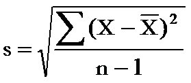
The equation for a sample standard deviation we just calculated is shown in the figure. Control charts are used to estimate what the process standard deviation is. For example, the average range on the X-R chart can be used to estimate the standard deviation using the equation s = R/d2 where d2 is a control chart constant (see March 2005 newsletter).
Use of Standard Deviation
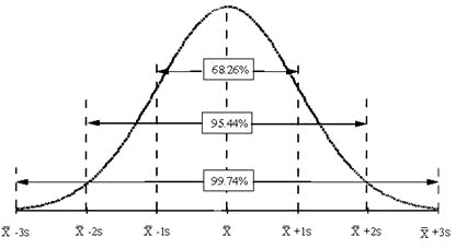
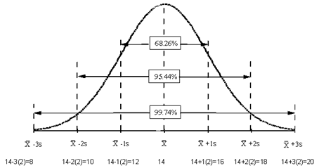
So, why are the standard deviation and, for that matter, the average important? There are many types of control charts that are based on variables data. The basic probability distribution that governs the calculation of the control limits on these charts is the normal distribution. The normal distribution is the familiar bell shaped curve shown in the above figure.
The normal distribution has several interesting characteristics. The shape of the distribution is determined by the average, X, and the standard deviation, s. The highest point on the curve is the average. The distribution is symmetrical about the average. Most of the area under the curve (99.7%) lies between -3s and +3s of the average. In addition, about 95.44% of the curve is between -2s and +2s of the average, while 68.26% of the curve is between -1s and +1s of the average.
To determine if a normal distribution exists, you can make a histogram of the individual results. If this histogram is bell-shaped, you can assume that the individual measurements are normally distributed. For example, suppose you are monitoring how long it takes to approve or disapprove a credit application for a customer. From your control charts (assume the process is in control), you have estimated the process average to be 14 working days and the standard deviation to be 2 days. After constructing a histogram on the days to approve or disapprove a credit application, you discover that it is bell-shaped. You can now replace the histogram with the normal distribution shown in the figure below.
Since the process is in statistical control, you know that about 67% of the time, it will take 12 to 16 days to process a credit application; 95% of the time it will take 10 to 18 days; and 99.7% of the time it will take 8 to 20 days. So, the average and standard deviation (for a normal distribution) allow you to begin to consider process capability. Can the process meet our customer specifications? Take a look at our three part newsletter on process capability.
