March 2019
(Note: all the previous SPC Knowledge Base in the basic statistics category are listed on the right-hand side. Select this link for information on the SPC for Excel software.)

Last month’s publication introduced nonparametric techniques for a single sample. This month, nonparametric techniques to compare independent samples are introduced.
In this issue:
Please feel free to leave a comment at the end of the publication. You can download a pdf copy of this publication here.
Nonparametric Techniques Review
Our SPC Knowledge Base has several publications showing how to analyze sample results. For example, you might want to test out two different supplier’s materials in your process. You take samples using both supplier’s materials and compare the results using a t-test for comparing the means of two processes. This type of test assumes you have a normal distribution.
Most of the time, the normality assumption is probably not thought about. It is simply ignored. There are times when you shouldn’t ignore this assumption. As noted in the last publication, there are lots of data that are not normal including lifetime data, call center waiting times, bacterial growth, or the number of injuries in a plant. You should not be using t-tests with these types of data.
The major difference between nonparametric techniques and those that require a normal distribution is the use of the median (μ ̃) instead of the average. The median provides a better estimate of the center of a non-normal distribution.
Two nonparametric techniques are described below. These deal with comparing independent samples. The Mann-Whitney test compares two independent samples. The Kruskal-Wallis test can be used with more than two independent samples. The general methodology for each technique is given below.
The example data and the mathematical equations to do the analysis come from the book “Statistics and Data Analysis: From Elementary to Intermediate” by Ajit Tamhane and Dorothy Dunlop.
Mann-Whitney Test
The Mann-Whitney test is used to determine if the observations from one population tend to be larger or smaller than another population. This is done by taking observations from each population. The assumption is that the two populations have the same shape, just different locations (e.g., different medians). In most cases, you will be testing the following hypothesis:
H0: θ1 = θ2
H1: θ1 ≠ θ2
where θ1and θ2are the location parameters for the two distributions.
The methodology involves comparing each observation from one distribution with each observation from the other distribution. It is easiest to understand this by looking at an example. These data are from the reference above. A company is interested in the failure time of a capacitor. They test 8 capacitors under normal conditions and then 10 capacitors under thermally stressed conditions. They want to find out if the thermally stressed conditions reduce the failure time. The data are shown below.
Table 1: Capacitor Failure Time Data
| Normal Conditions | Stressed Conditions |
|---|---|
| 5.2 | 1.1 |
| 8.5 | 2.3 |
| 9.8 | 3.2 |
| 12.3 | 6.3 |
| 17.1 | 7 |
| 17.9 | 7.2 |
| 23.7 | 9.1 |
| 29.8 | 15.2 |
| 18.3 | |
| 21.1 |
Note that this will be a one-sided test. So, the alternate hypothesis is H1: θ1 < θ2. Let the observations from the normal conditions be represented by xi and the observations from the stressed conditions be represented by yi. Let n1 be the number of observations for the normal conditions and n2 be the number of observations for the stressed conditions. The basic methodology is given below.
- Compare each xi to yi. Define u1= the number of pairs when xi > yi and let u2 be the number of pairs when xi < yi. There will be n1n2 comparisons with u1+ u2= n1n2.
- Reject H0 if u1 is large.
If you compare each of the values to each other, you get the following:
u1 = 59
u2 = 21
If the sample size is small, you use the null distribution to determine if u1 is large. You have to refer to a table that gives you the probabilities associated with the values of n1, n2 and u1. There is a table in the reference above. The p value from that table is 0.051.
If the sample size is large, you can approximate the null distribution using with normal distribution. In this case, you can calculate z using the following equation:
The calculated value of z is 1.643. You can use Excel’s NORM.S.DIST function to find the p value. The p value is 0.501, very close to the one from the table in the reference.
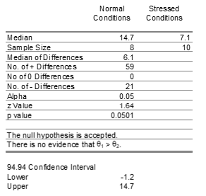
The output from the SPC for Excel software for the data in Table 1 is shown below.
The output gives the median of each of the two samples as well as the sample size. It gives the median of the differences (xi – yi) as well as the number of positive differences (u1) and the number of negative differences (u2). It also gives the number of ties, when xi = yi. When there is a tie, both u1 and u2 are increased by 1/2. Alpha in this example is 0.05. The software, for this data, uses the normal distribution approximation to the null distribution. The z value and the p value are given also. The confidence interval is also provided.
Note that the p value is 0.0501. This is larger than the alpha value of 0.05. So, if you have blinders on, you would accept the null hypothesis since the p value is larger than alpha. But there is essentially no difference between these two numbers. What should you do? Go get more data.
The p value is too close to alpha. So, in this example, there should be no clear conclusion.
Kruskal-Wallis Test
The Kruskal-Wallis test is used to compare multiple independent samples. Suppose there are k independent samples we want to compare. The following hypothesis is what we are testing:
H0: θ 1= θ2 = θ3…. = θk
H1: θi > θj for some i ≠ j
This methodology involves ranking all the observations in ascending order. The first observation is ranked 1, the second is ranked 2, etc. Then you sum the ranks by the sample and calculate an average rank for that sample. So, the methodology is looking for differences in the ranks for the various samples. There is a statistic called the Kruskal-Wallis statistic that is calculated. If it is large, then H0 is rejected. We will not show the details of the calculations here.
Consider the example from the reference above. Four different teaching methods are being compared. Test scores were collected for each teaching method. The data are shown in Table 2.
Table 2: Teaching Method Data
| Case Method | Formula Method | Equation Method | Unitary Analysis Method |
|---|---|---|---|
| 14.59 | 20.27 | 27.82 | 33.16 |
| 23.44 | 26.84 | 24.92 | 26.93 |
| 25.43 | 14.71 | 28.68 | 30.43 |
| 18.15 | 22.34 | 23.32 | 36.43 |
| 20.82 | 19.49 | 32.85 | 37.04 |
| 14.06 | 24.92 | 33.9 | 29.76 |
| 14.26 | 20.2 | 23.42 | 33.88 |
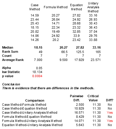
The analysis was performed using the SPC for Excel software. The output is shown below.
The output shows the original data and the median of each teaching method. The rank sum is then given along with the sample size and the average rank for each teaching method. The Kruskal-Wallis (kw) statistic is given along with the p value for that statistic. The p value is 0.0004, very small. So, the conclusion is that the teaching methods are not all the same – there are differences.
Pairwise comparisons are used to determine which teaching methods are different. That is the bottom part of the output. The pairwise difference is determined and compared to a critical value. Those with a pairwise difference greater than the critical value are significantly different. The “Case Method” and the “Formula Method” are both significant differently than the “Unitary Analysis Method” based on this output.
Summary
This publication has provided an overview of two nonparametric techniques. One was the Mann-Whitney test to compare two independent samples to see if one distribution tends to be greater or larger than the other distribution. The other was the Kruskal-Wallis test which looks at two or more distributions to see if any are different. Both methods are distribution-free methods. No assumption is made about the underlying distribution. The median is used as a measure of the center of the distribution.


