October 2016
(Note: all the previous SPC Knowledge Base in the basic statistics category are listed on the right-hand side. Select this link for information on the SPC for Excel software.)

You will not be able to calculate a Cpk value for the process capability – that calculation requires the data to be normally distributed. You are forced to do a non-normal process capability. Not the end of the world. A non-normal process capability requires determining what distribution best fits your data – and determining if there is a legitimate reason that your data follows that distribution.
Last month’s publication described how distribution fitting is done. This month’s publication describes how to compare the fit for various distributions to determine which distribution best fits your data. This in turn allows you to perform your non-normal process capability.
In this issue:
- Review of Distribution Fitting
- Our Data
- Distribution Fitting for Our Data
- Determining Which Distribution Fits Our Data Best
- Does the Distribution Make Sense for the Process?
- Application to Non-Normal Process Capability Analysis
- Summary
- Quick Links
Please feel free to leave a comment at the end of this publication. You may also download a pdf copy of this publication at this link.
Review of Distribution Fitting
Distribution fitting is the process used to select a statistical distribution that best fits a set of data. Examples of statistical distributions include the normal, Gamma, Weibull and Smallest Extreme Value distributions. In the example above, you are trying to determine the process capability of your non-normal process. This means that you need to be able to define which distribution fits the data best so you can determine the probability of your process producing material beyond the specifications. It is important to have the distribution that accurately reflects your data. If you select the wrong distribution, your calculations against the specifications will not accurately reflect what the process produces.
Various distributions are usually tested against the data to determine which one best fits the data. You can’t just look at the shape of the distribution and assume it is a good fit to your data.

The location parameter of a distribution indicates where the distribution lies along the x-axis (the horizontal axis). The scale parameter of a distribution determines how much spread there is in the distribution. The shape parameter of a distribution allows the distribution to take different shapes. The threshold parameter of a distribution defines the minimum value of the distribution along the x-axis. The four parameters were discussed in detail in our last publication.
A number of statistical techniques can be used to estimate the parameters for a distribution. SPC for Excel uses the maximum likelihood estimation (MLE) technique. In this process, parameters are chosen that minimize something called the negative log likelihood. An example of how this is done for the exponential distribution was given in last month’s publication. Once this estimation is complete, you use goodness of fit techniques to help determine which distribution fits your data best. There also visual techniques that help you decide which distribution is best. These includes examining a histogram with the distribution overlaid and comparing the empirical model to the theoretical model.
Our Data
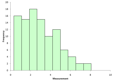
Suppose we have sample of 100 data points. You can download the data used at this link. A histogram (Figure 1) shows that the data are not normally distributed.
Figure 1: Histogram of Our Data
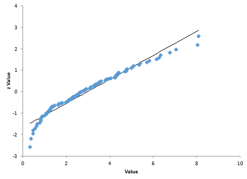
The normal probability plot is shown in Figure 2. The data do not lie close to the straight line. The p-value for the Anderson-Darling statistic is 0.01, which is small. This confirms that the data are not normally distributed. For more information on the normal probability plot and the Anderson-Darling statistic, please see this publication.
Figure 2: Normal Probability Plot of Our Data
Distribution Fitting for Our Data
The next step is to fit the data to various distributions. Most software packages have numerous distributions that can be tested against the data. SPC for Excel was used to fit the various distributions. The output will be shown in three parts. The first part shows the parameters that were estimated for each distribution using the MLE method. These parameters are given Table 1.
Table 1: Parameter Estimates from the Distribution Fitting
| Distribution | Location | Shape | Scale | Threshold |
| Weibull | 1.729 | 3.342 | ||
| Weibull – Three Parameter | 1.506 | 3.006 | 0.253 | |
| Gamma | 2.446 | 1.216 | ||
| Gamma – Three Parameter | 2.142 | 1.33 | 0.126 | |
| Largest Extreme Value | 2.145 | 1.424 | ||
| LogNormal – Three Parameter | 1.387 | 0.416 | -1.379 | |
| LogNormal | 0.872 | 0.719 | ||
| LogLogistic – Three Parameter | 1.309 | 0.27 | -1.058 | |
| LogLogistic | 0.933 | 0.411 | ||
| Exponential – Two Parameter | 2.646 | 0.329 | ||
| Normal | 2.975 | 1.78 | ||
| Logistic | 2.848 | 1.019 | ||
| Exponential | 2.975 | |||
| Smallest Extreme Value | 3.917 | 1.988 |
Not all distributions have the same parameters. For example, the normal distribution is described by the location and the scale while the Gamma distribution is described by the shape and scale. The parameters in Table 1 minimized the negative log-likelihood for each distribution. For the Weibull distribution, the shape parameter was estimated to be 1.729 and the scale parameter estimated to be 3.342. These two parameters minimized the negative log-likelihood for the Weibull distribution.
The data in Table 1 are actually sorted by which distribution fits the data best. The next section describes how this was determined.
Determining Which Distribution Fits the Data Best
The second part of the output is used to determine which distribution fits the data best. Table 2 shows that output. Each column is described below.
Table 2: Goodness of Fit Information by Distribution
| Distribution | Log-Likelihood | AD | p Value | LRT | AIC |
| Weibull | -190.3 | 0.237 | >0.25 | 384.6 | |
| Weibull – Three Parameter | -189.4 | 0.355 | >0.25 | 0.174 | 384.7 |
| Gamma | -191.1 | 0.462 | >0.25 | 386.2 | |
| Gamma – Three Parameter | -191.0 | 0.536 | 0.197 | 0.691 | 388.1 |
| Largest Extreme Value | -193.6 | 0.499 | 0.226 | 391.2 | |
| LogNormal – Three Parameter | -192.9 | 0.514 | 0.189 | 0.011 | 391.9 |
| LogNormal | -196.2 | 1.385 | 0.001 | 396.3 | |
| LogLogistic – Three Parameter | -195.9 | 0.684 | 0.044 | 0.109 | 397.8 |
| LogLogistic | -197.2 | 1.175 | <0.005 | 398.4 | |
| Exponential – Two Parameter | -197.3 | 3.875 | <0.001 | 0.000 | 398.6 |
| Normal | -199.5 | 1.029 | 0.010 | 403.1 | |
| Logistic | -200.5 | 0.881 | 0.012 | 405.0 | |
| Exponential | -209.0 | 6.374 | <0.001 | 420.0 | |
| Smallest Extreme Value | -216.1 | 3.357 | <0.01 | 436.2 |
The first column in Table 2 is the log-likelihood value. This is the minimum value for the given distribution based on the parameters in Table 1. Most software will not give this value. However, it is used here to determine the AIC value in the last column.
The second column lists the Anderson-Darling statistic. This statistic is used to help determine how good the fit is. The link above for the normal probability plot shows how the Anderson-Darling statistic is calculated for the normal distribution. The calculations are similar for the other distributions; you just use that distribution in place of the normal distribution. The statistic is calculated and the p-value associated with that statistic determined. The test assumes that the data fits the specified distribution. A low p-value means that assumption is wrong, and the data does not fit the distribution. A high p-value means that the assumption is correct, and the data does fit the distribution.
The p-values for the Anderson-Darling statistic are given in the third column. The p-values used in the software are taken or extrapolated from tables in the book “Goodness-of-Fit Techniques” by Ralph D’Agostino and Michael Stevens.
The fourth column lists the p-value for the likelihood ratio test (LRT). Look at Table 2. Note that there is only a LRT value when there are two distributions from the same family, e.g., the Weibull and the three parameter Weibull. In these cases, the second distribution is created by the addition of the threshold parameter. The LRT determines whether there is a significant improvement in fit with the addition of the threshold parameter.
The smaller the p-value in the LRT column, the more likely the addition of the extra parameter created a significant improvement in fit. The three parameter log-normal distribution has a value for 0.011 for LRT. This implies the extra parameter improved the fit. The three parameter Gamma distribution has a value of 0.691 for LRT. This implies that the extra parameter did not improve the fit significantly.
The fifth column contains the Akaike information criterion (AIC) value. AIC compares the relative “quality” of a model (distribution) versus the other models. You can use AIC to select the distribution that best fits the data. The distribution with the smallest AIC value is usually the preferred model. AIC is defined as the following:
AIC = 2k – 2(Log-Likelihood)
where k is the number of parameters. Note that the AIC value alone for a single distribution does not tell us anything. It is not a test like the p-value from the Anderson-Darling statistic. The AIC value compares the relative quality of all distributions. So, if all distributions do not fit the data well, the AIC value will not let you know this. You need to combine the p-values for the Anderson-Darling statistic, the LRT, and the AIC value to help determine which data fits the distribution best.
Based on the results, it appears that the Weibull and the three parameter Weibull both fit the data pretty well. The Smallest Extreme Value distribution fits the data the worst.
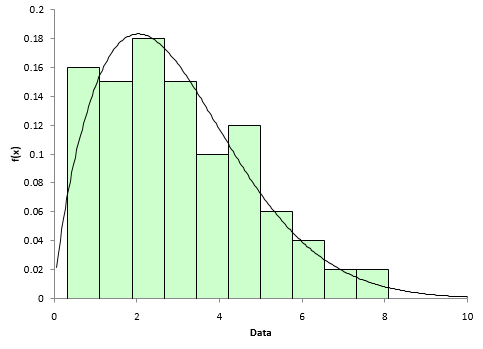
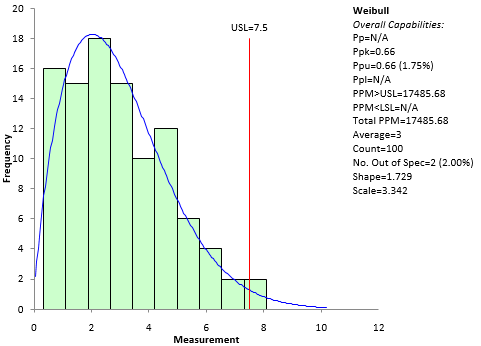
There are also visual methods you can use to determine if the fit is any good. One is to overlay the probability density function (pdf) for the distribution on the histogram of the data. Figure 3 shows this for the Weibull distribution. Note that the pdf does seem to fit the histogram – an indication that the Weibull distribution fits the data.
Figure 3: Histogram/pdf for Weibull Distribution Fit
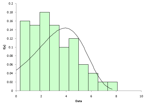
Figure 4 shows the histogram/pdf for the Smallest Extreme Value. The pdf does not appear to overlay the histogram very well – an indication that the Smallest Extreme Value distribution does not fit the data well.
Figure 4: Histogram/PDF for Smallest Extreme Value
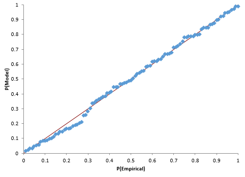
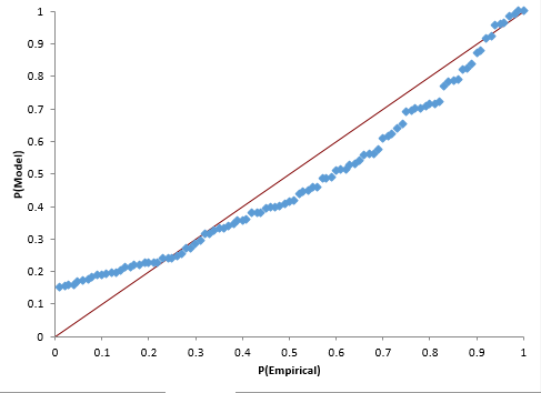
Another visual way to see if the data fits the distribution is to construct a P-P (probability-probability) plot. The P-P Plot plots the empirical cumulative distribution function (CDF) values (based on the data) against the theoretical CDF values (based on the specified distribution). If the P-P plot is close to a straight line, then the specified distribution fits the data.
Figure 5 shows the P-P plot for the Weibull distribution results. The points fall along the straight line indicating that the distribution does fit the data.
Figure 5: P-P Plot for Weibull Distribution Fit
Figure 6 shows the P-P plot for the Smallest Extreme Value results. Note that the points do not fall along the straight line – another indication that this distribution does not fit the data.
Figure 6: P-P Plot for Smallest Extreme Value Distribution Fit
Does the Distribution Make Sense for the Process?
You have determined which distribution fits your data best. This is an important step. It is easy to do with software. But you should have a reason for using a certain distribution – it must make sense in terms of your process. For example, the Weibull distribution is widely used in reliability and life data analysis. If this is the distribution that fits the data best, does it make sense in terms of your process? It may not always be possible to do, but you should have a reason to believe that the data fits a certain distribution – beyond the numbers saying this is the best distribution. In the example above, there is probably very little difference between how well the Weibull and Gamma distributions fit the data. Which one makes the most sense for your process?
Application to Non-Normal Process Capability Analysis
Now that it has been determined that the Weibull distribution fits the data best, we can perform a non-normal process capability analysis. A previous publication covered how to do this. The upper specification limit is 7.5; there is no lower specification limit. The SPC for Excel software was used to generate the non-normal process capability analysis. The chart is shown in Figure 7. It shows that the process has a Ppk = 0.66. Not where you want for your PPAP! Back to work on reducing variation in your process.
Figure 7: Process Capability Analysis Using the Weibull Distribution
Summary
This publication covered how to determine which distribution best fits your data. Distributions are defined by parameters. The maximum likelihood estimation method is used to estimate the distribution’s parameters from a set of data. Methods of checking how “good” the distribution matches the data were also introduced. These goodness of fit methods include the Anderson-Darling statistic, comparing the histogram to the probability density function, and constructing a P-P plot to compare the theoretical cumulative density function to the empirical cumulative density function. The Akaike information criterion (AIC) value was also introduced to determine of the quality of the distribution fit to the other distributions. The distribution with the lowest AIC value is usually the preferred distribution – as long as the Anderson-Darling statistic p-value is large.
A/C Goodness of Fit Information by Distribution HOW DO YOU GOT A NEGATIVE -190.3 i,e WEIBULL -LOGLIKELIHOOD (-190.3)
Please see this link: https://www.spcforexcel.com/knowledge/basic-statistics/distribution-fitting
You are working with -LN(L)
Firstly, thank you so much for this wonderful article that explains the procedure of determining the right distribution for a given set of data. I only have one question though. What is the connection between Table 1 and the set of values that has been presented in Table 2 ? For example, are the Goodness-of-Fit Test results for the different candidate distributions in Table 2 calculated based on the distribution parameters from Table 1 ?? Am I right to understand that the values presented in Table 2 couldn’t have been calculated without the data from Table 1 ?
Thank you for your kind words. You are correct. Table 1 gives the parameters for each of the distributions. Table 2 takes those parameters to determine goodness of fit, etc.
How can I determine which distribution fits my data the best in r programming? please help me to reach out of this point.
Sorry, I do not use R.
In R, use packages fitdistrplus and actuar, you find also examples in youtube (distributions fitting in R etc..)
Excellent article, sir. What should I do if my data distribution does not fit any of these standard curves? I used minitab and for all distribution p<0,005.
Did you try to transform the data using Box-Cox or the Johnson Transformations? If they don't work and none of the distributions fit, you are pretty much out of luck – what are you trying to do?
I tried to transform using box-cox and Johnson Transformation but both of the did not give a good fit.I have been trying to do a capability study for basis weight at a paper machine. Normally we just produce this special product with basis weight from 900-1000 for 2 days every month (every hour we take a sample to check the basis weigth). So I organized all the data from 2018 and 2019 (24 runs) in a spreadsheet and then realized that the distribution is not normal and with individual distribution identification I could not fit the data at any distribution available.Do you think the procedure is correct? What should I do? Thank you so much for the help
Is the process in control? If not, that is why the data may look non-normal. I quite often see that short runs start high or low for different runs – that might cause the histogram to look non-normal. Send me your data and i will take a look at it (bill@www.spcforexcel.com). If that is not the issue, I would just do a histogram and add specs to see if it looks like it is capable.
Many thanks for sharing this informative article. I was wondering how you calculated the LRT values?
Likelihood-ratio test statistic = 2 * L(A)- 2 * L(B).
where L(A) is the log likeihood for the three parameter distribution and L(B) is the log likelihood for the two parameter distribution. Use the chi-square distribution in Excel to define LRT:
LRT = chidist(likelihood-ratio test statistic, 1)
Excellent article, thank you so much
I would like to know below things on distribution analysis 1)When we have a large dataset with many features(many x variables–x1,x2,x3…) present in the whole data set then what is the approcah to determine the distribution?' 2) Should we find distribution for each variable separately and compare among themselves and process further to make them ditribution if they are not? 3) should we find distribution for only important variables and do the same thing if they are not ditributed well? 4)should we find distribution for Y(target) variable and do the same thing if they are not distributed well? 5) Should we find ditribution of x variables with relative to Target variable?
I am not sure what you are doing but I would find the distribution for each separate variable. I assume they are independent of each other.
I am trying to generate random data that follow a bimodal distribution. First, could you please explain the details of a bimodal distribution? Then, how to generate random data using this distribution. Lastly, how to identify if data follows bimodal distribution? Your reply will be greatly appreciated.
A bimodal distribution is one that has two peaks. Suppose you want to do this for a normal distibution. You can randomally generate numbers for the situation when the average = 100 and standard deviation = 10. Then generate another one with average of 80 and standard deviation 0f 10. You can use any values you want. Combine them and you have a bimodal distribution.
Very resourceful article. Could you be having a more detailed ebook about those concepts?
We would like to do that – just an issue of time. Thanks.