April 2019
(Note: all the previous SPC Knowledge Base in the basic statistics category are listed on the right-hand side. Select this link for information on the SPC for Excel software.)

That is what I would have done until I read an article from 2017 by Dr. Donald Wheeler and James Beagle III that described a new test for homogeneity. The problem with the XmR chart approach to doing this is that the number of data points sets the alpha level, which is the risk of a false alarm. This is different from “one-time” tests where you pick the risk of a false alarm. For example, in determining if the means of two processes are the same, you might select an alpha = 0.05. You can’t pick the alpha level with the XmR chart approach – it is set by the number of points used to set the control limits.
The publication described a new test for homogeneity. This test is called the Analysis of Individual Values (ANOX) and is presented in this publication. In this issue:
- Example Data
- XmR Chart Approach/Analysis of Individual Values (ANOX) Approach
- The Scaling Factors
- Summary
- Video: Analysis of Individual Values
- Quick Links
Please feel free to leave a comment below. You can download a pdf copy of this publication at this link.
Example Data
Suppose you have just finished a 125-piece PPAP of a new product for a customer. A key characteristic of the new product was measured on each of the 125 pieces. The data are shown below in Table 1.
Table 1: Example Data
| 105.4 | 94.7 | 94.6 | 114.0 | 96.5 |
| 100.8 | 103.1 | 97.0 | 103.4 | 99.7 |
| 102.0 | 103.8 | 94.8 | 103.3 | 89.9 |
| 94.5 | 93.7 | 116.3 | 98.2 | 99.4 |
| 94.8 | 94.2 | 120.5 | 87.1 | 93.5 |
| 102.3 | 109.5 | 97.5 | 101.5 | 103.3 |
| 67.2 | 109.3 | 94.1 | 105.1 | 101.1 |
| 101.2 | 102.3 | 90.1 | 132.4 | 89.9 |
| 108.9 | 122.0 | 90.2 | 109.7 | 115.4 |
| 105.5 | 113.5 | 103.8 | 80.0 | 104.0 |
| 83.1 | 92.5 | 97.7 | 101.1 | 100.2 |
| 97.8 | 105.1 | 97.8 | 113.8 | 97.2 |
| 110.9 | 132.1 | 105.6 | 98.2 | 87.6 |
| 108.1 | 101.3 | 95.5 | 104.6 | 107.9 |
| 96.8 | 100.9 | 103.4 | 100.1 | 99.0 |
| 117.7 | 101.2 | 91.9 | 100.3 | 106.9 |
| 131.4 | 132.5 | 91.1 | 99.1 | 102.4 |
| 99.4 | 104.6 | 102.1 | 96.2 | 109.7 |
| 116.4 | 67.9 | 86.0 | 97.6 | 79.2 |
| 96.5 | 101.9 | 98.9 | 93.9 | 91.9 |
| 100.6 | 87.2 | 113.1 | 84.1 | 85.5 |
| 107.3 | 87.4 | 93.6 | 93.1 | 87.5 |
| 83.9 | 108.4 | 107.9 | 120.4 | 95.6 |
| 102.3 | 94.3 | 96.9 | 84.5 | 88.7 |
| 99.2 | 83.1 | 94.5 | 97.2 | 65.1 |
You want to answer the question if the results are homogeneous. We will compare two approaches: the XmR control and ANOX. The approach below is based on the original article on the Analysis of Individual Values (ANOX), which was published by Quality Digest.
XmR Chart Approach
The first thing to realize is that using a XmR chart to determine if a dataset is homogenous is different from using a XmR chart to monitor a process over time. The latter is the normal use of an individuals control chart. If you are using a XmR chart to monitor a process over time, you collect baseline data. This is typically 17 to 30 points for the XmR chart. You then calculate the average and control limits, and if the process is in control, you set the average and control limits and monitor the process against them into the future.
You collect another data point and compare it to the baseline to see if it is significantly different. This is the sequential nature of using a control chart to monitor a process. Each additional point represents a test of whether the point is a signal or not. With 3 sigma limits, the probability of a false signal (alpha) is 0.0027 (based on the normal distribution). As shown below, this is not the alpha associated with a one-time test when using the XmR chart to check for the homogeneity of a dataset.
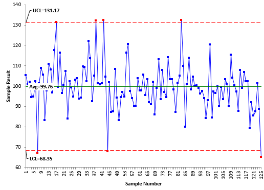
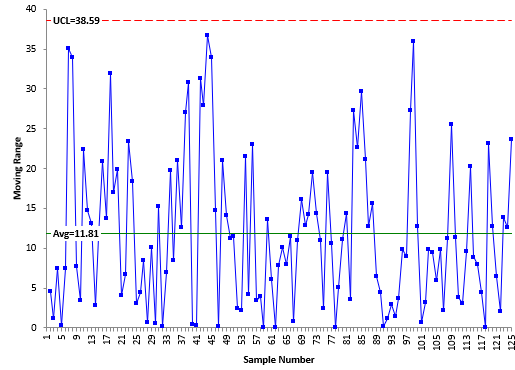
The data in the table above were analyzed using a XmR chart. The data is sequential by columns, i.e., the first column represents the first 25 data points, the second column the next 25 data points, etc. Figure 1 shows the X chart for the data. The moving range chart is shown in Figure 2.
Figure 1: X Control Chart
Figure 2: Moving Range Chart
The moving range chart is in statistical control. There are no points beyond the control limits. There are seven out of control points on the X chart. This would imply that the dataset is not homogeneous and contain outliers.
What about the level of alpha in the control chart above? Remember, this is a one-time test, not the usual sequential process of adding a data point and testing it against the baseline data. What is the risk of a false alarm when using these 125 data points as baseline data? The authors in the article referred to this as the “baseline alpha.” They used Bonferroni’s inequality to define the following:
1 – (1- alpha)k≤ baseline alpha ≤ k(alpha)
where k is the number of data points. For a normal distribution and the three-sigma limits on the XmR chart, the value of alpha is 0.0027. The baseline alpha is then given by:
1 – (1- 0.0027)125≤ baseline alpha ≤ 125(0.0027)
0.287 ≤ baseline alpha ≤ 0.338
This means that the risk of a false alarm is between about 29% and 34% when you use 125 data points and an XmR chart to decide about homogeneity.
Note that you did not get to choose the value of alpha – like you do on other one-time tests – like using a value of alpha = 0.05 to determine if there is a difference between means. Usually you want a higher alpha (0.10) if you want to reduce the risk of a missed signal or a smaller alpha (0.01) if you want to minimize the chance for a false signal. Wheeler and Beagle recognized this problem and proposed a different approach for analyzing the homogeneity of a dataset – particularly for larger datasets.
Analysis of Individual Values (ANOX) Approach
Suppose you have k individual values. You would like to know if the data are homogeneous. The ANOX approach is given by the following steps:
- Calculate the moving range for each successive difference between the individual values
- Calculate the average moving range
- Calculate the average of the k individual values
- Determine the alpha value (risk of false alarm)
- Determine the scaling factor ANOXα
- Calculate the upper and lower ANOX limits: average ± ANOXα(average moving range)
- Interpret the chart for homogeneity
Note that in this process, you select the value of alpha. The scaling factor above depends on alpha and the number of data points. Suppose you want to reduce the risk of a missed signal and set alpha to 0.10. In the article referenced above, the authors provide a table of scaling factors for values of k from 8 to 480 and alpha values of 0.01, 0.05 and 0.10. The value of ANOXαis 2.96 for alpha = .10 and k = 125. The ANOX limits are then:
average ± ANOXα(average moving range)
99.76 ± 2.96(11.81)
64.7 to 134.8
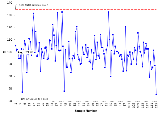
Figure 3 is the ANOX plot for this situation.
Figure 3 ANOX Chart
All the points on this chart are between the limits. This indicates that the data are homogeneous – a different conclusion than with the XmR chart.
A few observations about the ANOX chart. The alpha level associated with ANOX is the probability that either the minimum or maximum value will fall outside the limits. So, the 10% ANOX example above does not mean that 10% of the values will fall beyond the limits. It means that there is a 10% chance that the minimum or maximum value will fall beyond the limits. Also, a false alarm with the ANOX chart is usually a single point just beyond the limits. You still must make a judgement call about whether the data are homogeneous or not. In general, the more points beyond the limits and the further those points are from the limits, the more likely the data are not homogeneous.
The Scaling Factors
The article referenced above explains how the authors created the scaling factor tables for alpha values of 0.01, 0.05 and 0.10. The tables are available for download here.
Summary
This publication introduced the Analysis of Individual Values (ANOX) technique. This technique is used as a one-time test to determine if a dataset is homogeneous. It is particularly useful for larger datasets and allows you to select the alpha, the risk of a false alarm. The limits on the ANOX chart are based on the value of alpha selected and the number of data points you have.


Very informative and interesting