SPC and Selecting a Supplier

October 2015

Your company is pushing you for ways to decrease costs. Decreasing costs goes straight to the bottom line – or at least that is the thought process. A potential supplier has a new product for you to test. This new product costs more than the product you are using from your current supplier. The potential supplier claims this new product will work much better than your current product. How do you decide if you should switch to this new product? Not a good way of doing this without collecting data.

This month’s newsletter takes a look at how SPC can be used to help determine which supplier to select to use in the long term. The process starts with collecting baseline data on the existing supplier and then running tests using the potential supplier’s product. A control chart is used to compare the two suppliers. And then you have to do some calculations to determine the financial impact to your company.

The example in this publication involves saw blade life. One metric that be used to monitor saw blade life is called the G-ratio. This metric is used to compare two suppliers.

In this issue:

• Introduction
• G-Ratio
• Supplier A Baseline G-Ratio Data
• Supplier B G-Ratio Data
• Comparing the Cost of Supplier A to Supplier B
• Continued Monitoring
• Summary
• Quick Links

You may download of pdf copy of this publication here. Please feel free to leave a comment at the end of this publication.

Introduction

Your product is a steel bar. Part of your process involves cutting that steel bar to length using a saw. The saw blade wears down over time and eventually has to be changed when it is no longer cutting effectively. This results in some downtime. Plus, saw blades are expensive. So, the more saw blades you use, the higher your costs and the more downtime there is. You are currently using saw blades provided by Supplier A. Now, a potential supplier, Supplier B, has a new saw blade that costs more, but Supplier B claims that the new saw blade will cut much more bar than your existing saw blades.

What is your approach to compare Supplier A and Supplier B? Test out a few of the new saw blades from Supplier B and see if your operators think they perform better? That might work, but then again, it is not too data-based. You could measure how long a saw blade lasts from Supplier A and compare that to a saw blade from Supplier B. That is getting closer.

What you need in any analysis like this is a metric that allows you to compare the performance of the suppliers. A useful metric for saw blade life is the G-ratio. This is a measure how much material a blade can cut over its lifetime. The G-ratio calculation is explained below.

G-Ratio

The G-ratio can be used to compare saw blades (or other things like grinding wheels). The G-ratio is the ratio of the total area cut per blade to the area of the blade consumed. In this example, our product is a bar and is cut to length. The outer diameter (OD) of the bar is 1.8 inches. The bar radius (R)is then OD/2 = 0.9 The cross-sectional area of the bar can be calculated as:

Area = πR²= π(0.9)²= 2.545

Let k = number of cuts a saw blade makes. This saw blade makes 150 cuts. The total bar area cut is then given by:

Total Area Cut = k(πR²) = 150(2.545) = 381.75

To calculate the G-ratio, we still need the area of the saw blade consumed during cutting. The starting OD of the saw blade is 26 inches. After 150 cuts, the saw blade OD is 20.10 inches. The saw blade area used is given by:

Starting Area – Ending Area = π(26/2)²– π(20.10/2)²= 213.62

The G-Ratio is given by:

G-Ratio = Total Bar Area Cut/(Saw Blade Area Consumed) = 381.75/213.62 = 1.787

This value can be used to compare saw blade performance over time. The higher the G-ratio, the more bar area a saw blade can cut.

Supplier A Baseline G-Ratio Data

If baseline data does not exist for the current supplier, it has to be collected. Suppose you set up an Excel spreadsheet where your operators enter the bar OD, the number of cuts, the starting OD of the saw blade and the ending OD of the saw blade. You add the formula to calculate the G-ratio.

The operators collect the data for you over thirty samples. There are no problems with the data collection. The operators do a great job of remembering to enter the data and do so accurately. Happens all the time, right? Well, hopefully most of the time.

The data collected by the operators are given in the table below.

Table 1: Supplier A Baseline G-Ratio Data

The average of these thirty samples is 1.106. Do you now just test Supplier B’s test saw blades and compare averages? You could do that, but you might be missing a very important point – and that is statistical control. Is the process that generated the 30 results in Table 1 consistent and predictable? Or are there special causes present? If there are special causes present, then you don’t really know that the average is 1.106.

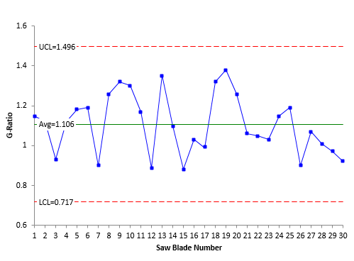
Only one way to check this and that is to use control charts. The individual control chart for the baseline G-ratio for Supplier A is shown in Figure 1. We will not show the moving range chart here.

Figure 1: X Chart for G-Ratio for Supplier A

The control chart in Figure 1 is in statistical control – the process for Supplier A appears to be consistent and predictable. Over time, the G-ratios will vary from about 0.72 to 1.5 with an average of 1.1.

Now you have your Supplier A baseline data. The average and the control limits based on the baseline data are used to judge if the saw blades from Supplier B have a significant impact on the G-ratio.

Supplier B G-Ratio Data

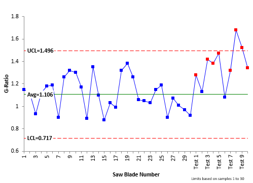
Supplier B has given you ten blades to test out. The ten blades are run in production and the operators collect the G-ratio data. The data are shown in Table 2. The data in Table 2 are added to the control chart as shown in Figure 2.

Table 2: Saw Blade G-Ratio for Supplier B

Figure 2: X Chart: G-Ratio with Test Blades Added

Remember that the average and control limits are based on the baseline data from Supplier A. You can see from Figure 3 that there are out of control points with the test saw blades from Supplier B. The points in red are out of control. The out of control conditions include one point beyond the control limit as well as Zone B test (4 out of 5 consecutive points in Zone B or beyond) and Zone A test (2 out of 3 consecutive points in Zone A or beyond). Please see our publication on interpreting control charts for more information on out of control tests.

It is clear from Figure 2 that the test saw blades from Supplier B have a higher G-ratio than the current saw blades from Supplier A. The control limits can be split starting with the first test saw blade. This was done and is shown in Figure 3.

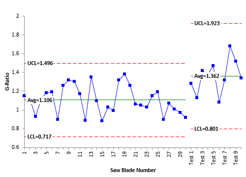
The G-ratios for the test saw blades from Supplier B appear to be in statistical control. There are no out of control points for the test saw blades. The average G-ratio for the test saw blades is 1.362. This compares to 1.106 for the current saw blades from Supplier A.

Supplier B definitely has a higher G-ratio than Supplier A. So, do you switch to Supplier B with the test saw blades? No, not quite yet. You need to look at the financial impact of switching.

Figure 3: X Chart with Split Control Limits

Comparing the Cost of Supplier A to Supplier B

The test saw blades performed better based on G-ratio. The ratio of the G-ratio for the test saw blade to the current saw blades is 1.362/1.106 = 1.24. This means that it will take 1.24 of the current saw blades from Supplier A to cut what one test saw blade from Supplier B will. Supplier A saw blades cost $50 each; Supplier B saw blades cost $70 each. So, 1.24 saw blades from Supplier A costs 1.24(50) = $62. This is less than the cost of the test blade from Supplier B. Despite the better performance in terms of G-ratio for Supplier B, it is less costly to stay with the current saw blades from Supplier A.

It should be noted that changing the saw blades more frequently with Supplier A does create more downtime. The downtime costs could be added to the financial analysis. But based solely on the cost of the saw blade and the G-ratio, it makes more sense to stay with the current saw blades from Supplier A.

Continued Monitoring

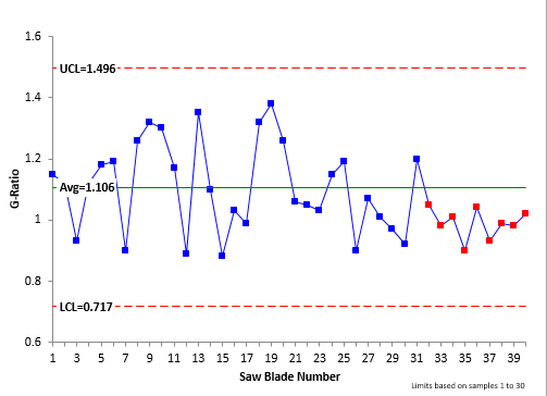
Saw blade life is an example of a real cost to an organization. The more saw blades you use, the more the cost. It makes sense to track performance of metrics like this over time. For example, suppose you continued to track the G-ratio over time for Supplier A. After time, the control chart looks like the one in Figure 4.

Figure 4: Control Chart for Supplier A Saw Blades

You can see what happened. The G-ratio has now decreased. Something with the supplier’s process has changed – and it is decreasing the cuts you get from each saw blade and increasing your costs. Time to talk to Supplier A.

Summary

This publication has looked at how control charts can be used to help select a supplier based on performance as well as overall cost. The key is to find a metric that reflects the performance you want. Collect the baseline data for one supplier and construct the control chart. If the process is out of control, you need to find out why and get the process into statistical control. Only then can you have faith in the results.

Then test the second supplier’s material. Use the control chart to search for differences between the suppliers. If the second supplier is significantly different, it will show up as out of control points on the control chart.

In addition to performance, you need to consider the overall cost to the organization of both suppliers.