March 2010
This is the third in a series of newsletters designed to introduce experimental design techniques.
In this newsletter, we will cover:
- Review Part 1
- Review Part 2
- Develop the regression model
- Use ANOVA to analyze the results
- Looking ahead
- Quick Links
The experimental design techniques we are examining are two-level full factorial designs. The newsletter series will show you how to plan, conduct and analyze these two level designs. A manual method of analyzing the results is given. This manual method provides clear method of understanding what an effect is, what a main effect is and what an interaction between factors is. We will use ANOVA (analysis of variance) in this newsletter to analyze the experimental design results. This is the most common way of examining the results of an experimental design with software that is available today.
Review of Part 1
You can read the first part at this link: part 1. In this first newsletter, we introduced the process we are using as an example of a two-level full factorial design. This process involves a stirred batch reactor. Your product is a chemical and the purity of that chemical is critical to customers. You would like to improve the chemical’s purity. There are two process variables that you think impact the purity: the reactor temperature and the residence time of the chemical in the reactor. How do you find out the following?
- Do the reactor temperature and/or residence time impact the average purity?
- If so, by how much? For example, if I change the reactor temperature 5 degrees, what is the impact on the average purity?
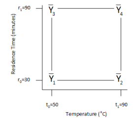
The experimental design space for this example is shown below. Reactor temperature has two levels: 50 and 90. Residence time also has two levels: 30 and 90. By running this design, we will be able to predict the results of purity anywhere in the design space with a minimum number of runs. This predictive ability of experimental design techniques is what makes them so powerful.
We then presented the data from our designed experiment. The data is shown below.
| Run | Rx. Temp. | Res. Time | % Purity | Average | Range | ||
| 1 | 50 | 30 | 74 | 78 | 73 | 75 | 5 |
| 2 | 90 | 30 | 65 | 64 | 69 | 66 | 5 |
| 3 | 50 | 90 | 74 | 76 | 78 | 76 | 4 |
| 4 | 90 | 90 | 85 | 88 | 91 | 88 | 6 |
We used the data to calculate the effects of each factor and interaction:
- Main Effect of Temperature = 1.5
- Main Effect of Residence Time = 11.5
- Interaction between Temperature and Residence Time = 10.5
A main effect is defined as the difference between the results when a factor is at its high level and when a factor is at its low level. Thus, purity is 1.5 higher at the high level of temperature than at the low level of temperature; it is 11.5 higher at the high level of residence time than at the low level of residence time.
The main effect describes how a factor influences a product response. This influence, however, sometimes depends on the levels of the other factors. This is called interaction. In this example, the interaction between temperature and residence time is 10.5. The next newsletter examined how to determine if these effects were significant.
Review of Part 2
You can read the second part at this link: part 2. The question is “are the main effects or interactions significant?” The answer is that it depends on the process variation. Replicating each treatment combination provides an estimate of the process variation. The process variation was estimated from a range chart. We used this estimate of the process variation to build confidence intervals around the two main effects and the interaction. The effect or interaction was considered significant if the confidence interval did not contain zero. The results showed the following:
- Factor B (residence time) and the interaction term AB were significant.
- Factor A (temperature) was not significant
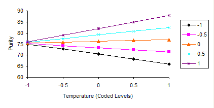
The results were graphed and are shown below.
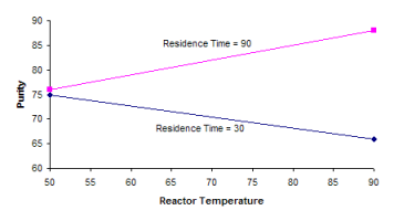
When residence time is at its low level (30), the purity decreases as temperature increases. However, when residence time is at its high level (90), the purity increase as temperature increases. Thus, there is a strong interaction between temperature and residence time.
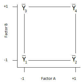
We then demonstrated how to use a design table to calculate the effects. To understand how to set up a design table, we used “coded” factor levels. When a factor is at its low level, it is represented by a -1. When a factor is at is high level, it is represented by a +1. This situation is shown in the figure below.
This design table can be used to determine the effects and interactions. This is demonstrated in the table below.
| Run | Mean | A | B | AB | Average |
| 1 | + | – | – | + | 75 |
| 2 | + | + | – | – | 66 |
| 3 | + | – | + | – | 76 |
| 4 | + | + | + | + | 88 |
| SPlus | 305 | 154 | 164 | 163 | |
| SMinus | 0 | 151 | 141 | 142 | |
| Overall | 305 | 305 | 305 | 305 | |
| Difference | 305 | 3 | 23 | 21 | |
| Effect | 76.25 | 1.5 | 11.5 | 10.5 |
To determine the values in the table:
- Enter the average response for each run under “Average.”
- Sum the average responses with + signs and enter the result in the row SPlus for each column.
- Sum the average responses with – signs and enter the result in the row SMinus for each column.
- Add SPlus and SMinus together and enter the result in the overall row for each column. This should be the same for each column.
- For each column, subtract SMinus from SPlus and enter the result in the difference row.
- Divide the difference by the number of + signs under the column to determine the effect.
Since we now know what effects are significant, we are ready to build the regression model.
Build the Regression Model
A regression model can now be developed based on this data. It assumes that there is no curvature in the design space. This means we are dealing with a linear model. This model makes use of the “coded” levels of the factors used in the design table. Remember that the high level of a factor was denoted by +1 in the design table, while the low level of a factor was denoted by -1. For a factor X, this is demonstrated in the figure below.
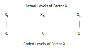
XL is the low level of Factor X, XM is the center point, and XH is the high level. The relationship between a coded level of Factor X, (Xc) and the actual level is given by the equation below.
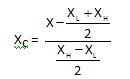
These coded factor levels are used in the regression model. For two factors and no curvature, the regression model is given by:
where Y is the response variable, b0 is the average of all experimental runs, b1, b2, b12 are half the calculated effects (retaining the sign) from the design table above, and x1 and x2 are the coded values for factors 1 and 2. Only effects that are significant are included in the model.
For the purity example, the effects of residence time and the interaction are the only significant effects. However, since temperature is part of the interaction, it is included in the model as well. The average of all runs was 76.25. Thus the regression model becomes:
Purity = b0 + b1x1 + b2x2 + b12x1x2 = 76.25 + 0.75A + 5.75B + 5.25AB
where A and B are the coded levels for factors A and B. This model can now be used to predict the responses for any setting of Factors A and B in the factor space, even though the runs may have never be made. This is demonstrated in the figure below. It is this predictive ability of experimental design that makes it such a powerful tool.
Based on this regression equation, the maximum purity will be obtained when both factors are at their high level. The purity at these factor levels can be predicted from the equation:
Y = 76.25 + 0.75A + 5.75B + 5.25AB = 76.25 + 0.75(+1)+ 5.75(+1) + 5.25(+1)(+1) = 88.0
ANOVA to Analyze the Experimental Design Results
ANOVA is commonly used to analyze the experimental design results with the software available today. Below the ANOVA table for this design that was generated from the SPC for Excel software.
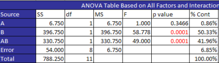
The columns are described below;
- Source: the source of the variation. For this example, the sources are A, B, AB, the error and the total.
- SS: sum of squares – a measure of the variation associated with the source
- df: degrees of freedom associated with the source
- MS: mean square = SS/df for each source
- F: F value for each source compared to mean square error
- p value: significance; if p is less than 0.05, the source is statistically significant
- % Cont: percent contribution of each source to the total sum of square
As can seen from the ANOVA table, the sources B and AB are significant. This agrees with our analysis using the design table. For more information on ANOVA, please see our single factor ANOVA newsletter.
You can also calculate the sum of squares from the design table. The sum of squares for each term is equal to the number of replications*difference^2 divided by the number of cells.
Looking Ahead
Next month we will take a look at how these techniques are used in the pharmaceutical industry. We will welcome back our guest author Nabil B. Darwazeh, Ph.D. He will take through an example that will introduce more details about experimental design techniques.