October 2009
In this issue:
- The Guest Author
- Introduction
- Case Study
- Statistical Analysis
- Bonferroni’s and Modified Levene’s Methods
- Process Control Charts
- Acceptance Chart
- References
- Quick Links
The Guest Author
 This month’s newsletter is the second written by Nabil B. Darwazeh, Ph.D. His first newsletter was last month’s entitled SPC and Pharmaceutical In-Process Control.
Dr. Darwazeh is currently a Research and Development Technical Advisor and Process Scale-Up Manager at United Pharmaceutical, Amman, Jordan. Before Joining United Pharmaceutical, he was Senior Research Scientist at Wyeth Pharmaceuticals, Pearl River, NY, and Research Scientist at Mallinckrodt Veterinary, Mundelein, IL.
He received his Bachelor’s Degree in Agriculture Sciences from University of Baghdad in 1980, and his Master’s Degree in Animal Science from California State University in 1983. Dr. Darwazeh received the Ph.D. Degree in Medicinal Chemistry and Pharmaceutical Sciences from University of Kentucky in 1995. Dr. Darwazeh is a member of the International Society for Pharmaceutical Engineering (ISPE). A special thanks to Dr. Darwazeh for sharing his insights into the use of SPC in the pharmaceutical industry.
Introduction
In-process raw materials and intermediates should be monitored, tested, and controlled during various steps of the pharmaceutical product manufacturing. This continuous monitoring and control is to identify and control expected and unexpected source of variations that might influence the finished product quality characteristics.
As an example, consider the case of the tablet hardness that was presented in the previous newsletter (September 2009). The major quality attribute “Tablet Hardness” is a critical concern to the quality assurance department. It reflects that the ingredients are adequately and uniformly blended, and particle segregation does not occur. Additionally, it assures that the compression process is constant during the time the powder mix was compacted into tablets.
This month newsletter focuses on a second quality attribute: Uniformity of Pharmaceutical Dosage Units. This quality characteristic must be monitored and controlled to provide enough assurance that the manufacturing process is under control.
According to the United States Pharmacopial (USP)1, the uniformity of dosage units can be demonstrated by either Content Uniformity (CU) or Weight Variation. Tablet content uniformity is defined by the USP as the degree of uniformity in the amount of drug substance among the dosage units. In this presentation, we will consider the CU as the estimate of the Uniformity of the Dosage Unit. The CU is based on the assay of the drug substance in a number of the individual dosage units to determine whether the individual content (expressed as percent of label claim) is within the limits set.
In the previous newsletter, we utilized statistical analysis in the form statistical control charts to demonstrate that the tablet compression process was under control with some variability. We achieved that by implementing the principles and methods of statistical process control to identify process operating and warning limits.
Our objectives of this month’s newsletter are implementing the same statistical principles provided by SPC for Excel V 4.0 Software to:
- identify the CU process limits
- use those process limits to determine the final product release specifications while monitoring the manufacturing process.
This approach allows us to identify unusual patterns of variability that may appear during process and the time at which this variation occurs.
Case Study
 Sequential (fractions) tablet samples were collected during tablet compression process according to procedure designated by US FDA as stratified sampling2. According to the US FDA Guidance, stratified sampling is defined as the process of sampling dosage units at predefined intervals and collecting representative samples from specific targeted locations in the compression operation that has greatest potential to yield highs and lows in test results.
In this process, 20 consecutive fractions of 10 tablets each were collected at predefined time-intervals during the compression process. Assay of the active drug substance in each individual tablet was performed using valid analytical method to assess the CU as percent of the label claim. Table 1 displays the assay results of individual tablets from the 20 consecutive fractions (F1, F2, etc.). Fraction averages, ranges and standard deviations are shown in Table 2.
| F1 | F2 | F3 | F4 | F5 | F6 | F7 | F8 | F9 | F10 |
| 98.3 | 102.9 | 109.7 | 101.2 | 98.3 | 100.3 | 105.8 | 100.5 | 91.6 | 106.0 |
| 102.5 | 98.7 | 93.8 | 103.1 | 105.4 | 106.0 | 96.2 | 94.9 | 91.4 | 96.5 |
| 108.7 | 101.7 | 107.0 | 98.4 | 94.2 | 100.5 | 108.9 | 96.1 | 91.3 | 90.4 |
| 103.5 | 96.4 | 100.2 | 101.5 | 103.9 | 100.7 | 101.6 | 96.0 | 97.7 | 102.7 |
| 96.9 | 103.2 | 104.2 | 99.1 | 106.4 | 109.0 | 109.6 | 95.7 | 105.6 | 96.2 |
| 100.4 | 96.9 | 100.6 | 95.7 | 99.9 | 91.9 | 101.9 | 100.5 | 100.7 | 109.0 |
| 106.0 | 113.0 | 99.3 | 112.9 | 103.2 | 91.4 | 95.2 | 86.9 | 107.5 | 104.5 |
| 100.6 | 103.5 | 104.4 | 106.2 | 113.0 | 91.3 | 107.0 | 96.5 | 96.5 | 106.0 |
| 93.8 | 96.2 | 103.4 | 91.6 | 109.7 | 97.7 | 107.0 | 100.2 | 104.2 | 100.6 |
| 94.0 | 104.5 | 94.5 | 96.9 | 94.7 | 105.6 | 103.1 | 106.6 | 107.8 | 105.0 |
| F11 | F12 | F13 | F14 | F15 | F16 | F17 | F18 | F19 | F20 |
| 100.5 | 100.7 | 109.0 | 91.9 | 94.9 | 91.3 | 97.7 | 105.6 | 108.0 | 105.7 |
| 96.5 | 111.6 | 96.4 | 106.0 | 104.5 | 98.3 | 104.6 | 94.1 | 93.6 | 104.7 |
| 93.8 | 102.9 | 106.2 | 103.5 | 96.5 | 102.5 | 95.8 | 96.2 | 101.8 | 106.8 |
| 94.0 | 104.5 | 107.5 | 109.7 | 105.6 | 108.7 | 106.4 | 94.9 | 113.8 | 104.1 |
| 101.7 | 96.4 | 103.2 | 96.9 | 113.0 | 103.5 | 96.2 | 104.5 | 105.7 | 106.3 |
| 91.9 | 91.4 | 91.3 | 97.7 | 109.7 | 96.9 | 99.9 | 96.5 | 87.2 | 100.5 |
| 104.6 | 101.5 | 99.0 | 96.5 | 94.7 | 104.0 | 100.2 | 105.6 | 104.4 | 98.1 |
| 109.6 | 99.1 | 99.1 | 87.2 | 97.9 | 99.9 | 93.6 | 100.6 | 97.0 | 95.4 |
| 99.3 | 95.7 | 90.4 | 95.4 | 105.8 | 87.3 | 101.8 | 102.8 | 102.2 | 108.3 |
| 99.0 | 112.9 | 106.1 | 97.5 | 101.3 | 101.2 | 106.8 | 102.7 | 99.4 | 102.8 |
| Fraction | Average | Sigma | Range |
| F1 | 100.47 | 4.89 | 14.9 |
| F2 | 101.70 | 5.09 | 16.8 |
| F3 | 101.71 | 5.08 | 15.9 |
| F4 | 100.66 | 5.92 | 21.3 |
| F5 | 102.87 | 6.15 | 18.8 |
| F6 | 99.44 | 6.38 | 17.7 |
| F7 | 103.63 | 4.99 | 14.4 |
| F8 | 97.39 | 5.12 | 19.7 |
| F9 | 99.43 | 6.68 | 16.5 |
| F10 | 101.69 | 5.74 | 18.6 |
| F11 | 99.09 | 5.40 | 17.7 |
| F12 | 101.67 | 6.76 | 21.5 |
| F13 | 100.82 | 6.66 | 18.6 |
| F14 | 98.23 | 6.63 | 22.5 |
| F15 | 102.39 | 6.36 | 18.3 |
| F16 | 99.36 | 6.30 | 21.4 |
| F17 | 100.30 | 4.58 | 13.2 |
| F18 | 100.35 | 4.53 | 11.5 |
| F19 | 101.31 | 7.54 | 26.6 |
| F20 | 103.27 | 4.11 | 12.9 |
Statistical Analysis
In pharmaceutical tablet production, the main concerns of the production and quality departments are:
- Are the means of all fractions equal?
- Are the variances of all fractions equal?
Answering the above questions is important if we would like to consider the homogeneity of the product output throughout the compression process. Large variability in both means and variances makes the determination of the finished product releases specifications difficult and unreliable.
There are a number of ways to answer the two concerns above. One method involves using statistical techniques that compare multiple means or variances at the same time. In this presentation, we will use Bonferroni’s method to compare multiple means and Modified Levene’s test to compare the variances. Please see our past newsletter for more information on Bonferroni’s method (January 2009). Another method to answer the two concerns is through the use of control charts. This will also be examined below.
Bonferroni’s and Modified Levene’s Methods
Therefore, we first evaluated the means of all fractions using Bonferroni’s method. Table 3 shows the analysis of variance of the multiple mean comparisons using alpha = 0.05.
Table 3: ANOVA for Bonferroni’s Method
| Source | Sum of Squares | Degrees of Freedom | Mean Square | F | p Value |
| Treatments | 519.0618 | 19 | 27.319042 | 0.81 | 0.6957 |
| Error | 6085.694 | 180 | 33.809411 | ||
| Total | 6604.756 | 199 |
The above ANOVA table provides the sum of squares of the treatment (fractions), error and total. It is clear that the probability value (p) is larger than the alpha value (0.05), therefore, the test for equal means does not show that there is evidence that any pairs of means are significantly different from each other. You can assume that all the fraction means are statistically the same. The software also compares each possible combination of the 20 fractions (190 comparisons in all). Each confidence interval contained zero confirming that there are no significant differences in the fraction means.
Next, we evaluated the variances of the fractions. Levene’s test offers a robust procedure because it is less likely to reject a true hypothesis of equality of variances just because the distributions of the sampled populations are not normal. SPC for MS Excel V4.0 software package is used to conduct the equal variance test. The assumption we are making to conduct this test is that each fraction represents a population of tablets and we collected random samples from all populations (fractions).
The null hypothesis to conduct this test is that the variances are equal:
where σi2represents the variance for fraction i and k is the number of fractions. The alternative hypothesis (H1) is that at least one variance is different.
The results for the Modified Levene Test are given below:
F Levene: 0.47
F Critical: 1.64
p Value: 0.9728
Since the p value is larger than 0.05, we can conclude that the variances of the 20 fractions are statistically the same.
Process Control Charts
The procedures above established that the fraction averages and variances are statistically the same. This provides the initial assurance that the compression process is stable. One may also reach the same conclusion using control charts. And the control charts provide a much more visible picture. The figure below is the Xbar control made using the SPC for Excel software.
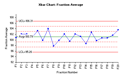
The chart above shows that all fraction averages are within Zone B (2 sigma) – an indication there are no special causes present. Also, the lack of trends suggests that the process is in statistical control. This also means that there are no statistically significant differences in the fraction means.
The range chart for the data is shown below.
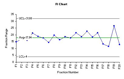
The range chart indicates that the variability of the process is quite stable and all fraction ranges are close to the overall range average. However, fraction 19 shows the highest range when compared to the remaining fractions. Inspection of the individual assay results of the ten tablets in fraction 19 shows that the wider range was caused by presence of highest assay value 113.8% and the lowest assay value 87.2. In pharmaceutical practices, it is not uncommon to face such variability at early stage of process optimization.
Process variability can further be monitored by assessing the behavior of the fraction standard deviations in an s control chart. One advantage of using fraction standard deviations (s) is that this s chart considers all data points involved in construction of any control chart.
The figure below is the s chart for the fraction standard deviations. Three lines are plotted on this chart as well. The middle line is the average standard deviation (sbar). The other two lines are the upper and lower control limits for the subgroup standard deviations.
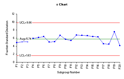
The tablet compression process variability depicted by the above s control charts demonstrates an example of a process that is in statistical control and the variability between the individual fractions is consistent over time.
Acceptance Chart
This part of the presentation deals with the determination of the initial in-house specifications for tablet CU assay3. The pharmaceutical manufacturing process varies from time to time within pre-specified limits. These limits are defined as follows:
- Acceptable Process Levels (APL): The process level at which it is acceptable and should be accepted most of the time
- Rejectable Process Levels (RPL): The process level at which it is rejectable and should be rejected most of the time
In the current case study, we decided to have Acceptable Process Levels (APL) of tablet CU assay between 97 and 103% of the label claim and Rejectable Process Levels (RPL) with limit of 2.5% above and below the APL:
APL(L) = 97%
APL(U) = 103%
RPL(L) = 97(1 – .025) = 94.58%
RPL(U) = 103(1+0.025) = 105.58%
The first step in constructing two-sided acceptance chart is to determine the sample size as in the following equation3:
where:
- σ: Population standard deviation of the process (unknown); replaced by sample standard deviation (s).
- Z(1/2σ) + Z(β): The (1/2σ)th and βth quantiles of a standard normal distribution. Since the population standard deviation (σ) is unknown, the quantiles of a standard normal distribution are replaced with those of a central t distribution with n-1 degrees of freedom.
It follows that the sample size for the lower and upper acceptance limits can be calculated as follows;
s was calculated from the range chart using s = (Rbar/d2), where d2 is a control chart constant that depends on subgroup (fraction) size. In this case, the fraction size is 10.
The sample size of 45 is used to calculate the lower and upper control level (ACL) based on APL using the following equations3:
ACL(L)= PAL(L)– [Z(α)(s) / (N)1/2] = 97 – [(1.96)(5.83) / (45)1/2] = 95.30
ACL(H)= PAL(L)– [Z(α)(s) / (N)1/2] = 103 + [(1.96)(5.83) / (44)1/2] = 104.72
The central line is the average of ACL(L) and ACL(U) which is 100.0 A new acceptance chart was constructed using the new value of the average and the acceptance limits. These values were manually entered into the control limit options of the Xbar control chart dialog box. The following Xbar control chart was generated using SPC for MS Excel software package.
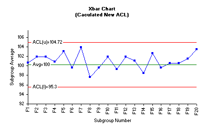
The acceptance Xbar control chart clearly depicts that no fraction average is outside the ACLs. Consequently, we conclude that the current tablets compression process resulted in a product that meets the in-house specifications. Based on all information generated in this practice, we can practically and safely revise the in-house specifications to a target value of average 100% of label claim and upper and lower rejectable limits of 95% and 105% respectively.
The above example has been very informative demonstration of the application statistical process control tools in monitoring the quality manufacturing process and science-based approaches to derive the final product specifications to meet the consumer requirements.
References
- “<905> Uniformity of Dosage Unit” in USP 32-NF27 (The United State Pharmacopeial Convention, Inc., Rockville, MD, 2009).
- Guidance for Industry. Powder Blends and Finished Dosage Units – Stratified In-Process Dosage Unit Sampling and Assessment (draft Guidance). US FDA, CDER October 2003.
- S.C. Chow, and J.P. Lui, “Quality Assurance” in Statistical Design and Analysis in Pharmaceutical Sciences: Validation, Process Controls, Practical and Clinical Application (Mercel Dekker, Inc., New Your, 1995), PP. 235-270.