June 2010
This is the second newsletter on attribute Gage R&R studies. As stated last month, sometimes a measurement system has a measurement value that comes from a finite number of categories. The easiest one of these is a go/no go gage. This gage simply tells you if the part passes or it fails. There are only two possible outcomes. In the last newsletter, we use a simple go/no go gage to demonstrate how to compare the appraisers. We used cross tabulation tables and calculated kappa values to compare the appraisers.
In this newsletter, we will
- Develop confidence intervals for % agreement for each appraiser
- Calculate the system effectiveness
- Compare each appraiser’s results to the reference value
- Draw conclusions based on the appraiser’s effectiveness, miss rate and false alarm rate
In this issue:
- Example
- Confidence Interval for Appraisers
- System % Effectiveness Score
- The Reference Values
- The Reference Values and Cross-Tabulation Tables
- The Reference Values and Kappa Values
- The Reference Values and Confidence Intervals
- The Reference Values and the System Effectiveness Score
- Conclusions
- Quick Links
Some of us use the manual Measurement Systems Analysis to help us understand our Gage R&R studies. This newsletter is a summary of their information contained in the third edition of the manual but provides more details of the calculations contained in the manual. Of course, our SPC for Excel software performs all the calculations automatically for you. Note that the fourth edition of Measurement Systems Analysis is now available, but the author has not yet reviewed it.
Example
The example was introduced in last month’s newsletter. Suppose you are in charge of a production process that makes widgets. The process is not capable of meeting specifications. You produce widgets that are out of specification. The process is in control and, as of yet, your Black Belt group has not figured out how to make it capable of meeting specifications. Your only alternative, at this time, is to perform 100% inspection of the parts and separate the parts that are within specifications from those that are out of specifications.
You have selected an attribute go/no go gage to use. This gage will simply tell if the part is within specifications. It does not tell you how “close” the result is to the nominal; only that it is within specifications.
To determine the effectiveness of the go/no gage, you decide to conduct an attribute gage R&R study. You select three appraisers (Bob, Tom and Sally). You find 30 parts to use in the trial. Each of these parts was measured using a variable gage and rated as passing (within specifications or conforming) or failing (out of specification or nonconforming). There are 21 conforming parts and 9 nonconforming parts in the study.
Each appraiser measures each part three times using the go/no go gage and the results are recorded. The parts must be run in random order without the appraiser knowing which parts he/she is measuring. In other words, randomize the 30 parts and have an appraiser measure each part. Then randomize the order again and repeat the measurement.
The results from the study are shown below. P indicates the part passed (conforming), while F indicates that the part failed (nonconforming). The first column is the reference value for the part. It represents the “true” value of the part based on the variable gage measurements.
Table 1: Attribute Gage R&R Study Results
| Appraiser |
Bob |
Bob |
Bob | Tom | Tom |
Tom | Sally |
Sally |
Sally |
|
| Reference |
Part/Trial | 1 | 2 | 3 | 1 | 2 | 3 | 1 | 2 | 3 |
| P | 1 | P | P | P | P | P | P | P | P | P |
| P | 2 | P | P | P | P | P | P | P | P | P |
| F | 3 | F | F | F | F | F | F | F | F | F |
| F | 4 | F | F | F | F | F | F | F | F | F |
| F | 5 | F | F | F | F | F | F | F | F | F |
| P | 6 | P | P | F | P | P | F | P | F | F |
| P | 7 | P | P | P | P | P | P | P | F | P |
| P | 8 | P | P | P | P | P | P | P | P | P |
| F | 9 | F | F | F | F | F | F | F | F | F |
| P | 10 | P | P | P | P | P | P | P | P | P |
| P | 11 | P | P | P | P | P | P | P | P | P |
| F | 12 | F | F | F | F | F | F | F | P | F |
| P | 13 | P | P | P | P | P | P | P | P | P |
| P | 14 | P | P | F | P | P | P | P | F | F |
| P | 15 | P | P | P | P | P | P | P | P | P |
| P | 16 | P | P | P | P | P | P | P | P | P |
| P | 17 | P | P | P | P | P | P | P | P | P |
| P | 18 | P | P | P | P | P | P | P | P | P |
| P | 19 | P | P | P | P | P | P | P | P | P |
| P | 20 | P | P | P | P | P | P | P | P | P |
| P | 21 | P | P | F | P | F | P | F | P | F |
| F | 22 | F | F | P | F | P | F | P | P | F |
| P | 23 | P | P | P | P | P | P | P | P | P |
| P | 24 | P | P | P | P | P | P | P | P | P |
| F | 25 | F | F | F | F | F | F | F | F | F |
| F | 26 | F | P | F | F | F | F | F | F | P |
| P | 27 | P | P | P | P | P | P | P | P | P |
| P | 28 | P | P | P | P | P | P | P | P | P |
| P | 29 | P | P | P | P | P | P | P | P | P |
| F | 30 | F | F | F | F | F | P | F | F | F |
Confidence Interval for Appraisers
Most software packages will calculate a confidence interval for each appraiser to show how well the appraiser agrees with himself/herself on all trials. We will demonstrate the calculations using Bob’s data. The first step is to determine how frequently Bob agrees with himself – that is, how often did Bob rate each part the same for each of the trials?
Looking through Table 1 for Bob’s data, you can see that there were 25 times Bob rated the part the same each time. There were five times when Bob did not rate the part the same each time (for parts 6, 14, 21, 22, and 26). This represents a percent agreement of 25/30 = 83.3%. So, Bob rated each part the same each time 83.3%. If we repeated this study, would Bob have this same percentage agreement? We don’t know but probably not because there are common causes of variation always present. We can develop a confidence interval around this average to give us an idea of the amount of possible variation in Bob’s results.
First, let’s define the following:
- m = number of times the each part was rated the same
- N = total number of parts
The calculations for the 95% confidence interval for the % agreement are given below. The F distribution is used to determine the confidence interval.
The lower confidence interval is given by the equation:
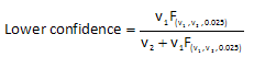
where:
- v1 = 2m
- v2 = 2(N-m+1)
- F = 2.5 percentile of the F distribution corresponding to v1 and v2 degrees of freedom.
From Bob’s data:
- v1 = 2m = 2(25) = 50
- v2 = 2(N-m+1)= 2(30-25+1) = 12
- F = 0.4512 (for alpha = 0.05 with 50 and 12 degrees of freedom)
You can find the value for F in statistical tables. You can also use the FINV function in Excel. But be aware that this function returns the inverse of the right-tailed F probability distribution. You want the left-tail so you would need to enter FINV(0.975, 50, 12) to get the correct tail portion. Excel 2010 has a new function F.INV which returns the inverse of the left-tailed F probability distribution. If you have Excel 2010, you can use F.INV(0.025, 50, 12) to get the F value.
The lower confidence limit is then:
Lower confidence = 50(0.4512)/(12+50(0.4512)) = 0.653 = 65.3%
The upper confidence limit is given by the following equation:
![]()
where:
- v1 = 2(m+1)
- v2= 2(N-m)
- F = 97.5 percentile of the F distribution corresponding to v1 and v2 degrees of freedom
From Bob’s data:
- v1 = 2(m+1) = 2(26) =52
- v2 = 2(N-m) = 2(5) = 10
- F = 3.216 (for alpha = 0.05 with 52 and 10 degrees of freedom)
The upper confidence is then:
Upper confidence = 52(3.216)/(10+52(3.216)) = 0.944 = 94.4%
Thus, the 95% confidence interval for Bob’s percent agreement is 65.3% to 94.4%. The confidence intervals for all three appraisers are given in the table below.
| Bob | Tom | Sally | |
| Total Inspected (N) | 30 | 30 | 30 |
| Number Matched (m) | 25 | 26 | 23 |
| 95% Upper | 94.4% | 96.2% | 90.1% |
| % Agreement | 83.3% | 86.7% | 76.&% |
| 95% Lower | 65.3% | 69.3% | 57.7% |
Since the % agreement for each appraiser lies in the confidence interval for each other appraiser, we must conclude that there is no statistically significant difference between the three appraisers.
System % Effectiveness Score
You can also determine an overall effective score for all three appraisers. The calculations are the same as for the confidence interval. The difference is that you first start by determining the number of parts where all three operators agreed on all trials, i.e., all operators rated the part the same for each trial – either a pass or fail. As shown in the data in first table, this occurred for 22 parts. There were 8 parts where the appraisers disagreed for some trial or trials. Thus, the overall % agreement is given by:
Overall % agreement = 22/30 = 0.733 = 73.3%
The 95% confidence interval for the overall agreement is calculated as shown above. The 95% confidence interval for the overall agreement is 54.1% to 87.7%.
The Reference Values
The first column in Table 1 contains the “Reference” value. This is the “true” value of the part as determined by a variable measurement system. The reference value can be used in the calculations in this newsletter (and the last one) by considering those results to be like another appraiser.
The Reference Values and Cross-Tabulation Tables
Thus, we can construct cross-tabulation tables (as shown in the last newsletter) that compare the results for each individual appraiser to the reference. The cross-tabulation table for Bob is shown below.
Table 3: Cross-Tabulation Table for Bob and the Reference
| Reference | |||||
| Fail |
Pass |
Total |
|||
| Bob |
Fail |
Count |
25 | 3 | 28 |
| Expected |
8.4 | 19.6 | 28 | ||
| Pass |
Count |
2 | 60 | 62 | |
| Expected |
18.6 | 43.4 | 62 | ||
| Total | Count |
27 | 63 | 90 | |
| Expected |
27 | 63 | 90 | ||
The cross-tabulation table simply organizes the results to make it easier to see if there are significant differences. Consider the rows labeled “Count.” The following is true from the table:
- Bob failed the part 25 times when the reference value was “Fail”
- Bob failed the part 3 times when the reference value was “Pass” (this is known as false alarm)
- Bob passed the part 2 times when the reference value was “Fail” (this is known as a miss)
- Bob passed the part 60 times when the reference value was “Pass”
Thus, Bob made the correct decision 85 times out of 90. The row labeled “Expected” are the expected accounts. This is the count you would expect if there was no difference between the appraiser and the reference.
The cross-tabulation tables for Tom and Sally are shown below. Tom made the correct decision 86 out of 90 times. Sally made the correct decision 79 out of 90 times.
Table 4: Cross-Tabulation Table for Tom and the Reference
| Reference | |||||
| Fail |
Pass |
Total |
|||
| Tom |
Fail |
Count |
25 | 2 | 27 |
| Expected |
8.1 | 18.9 | 27 | ||
| Pass |
Count |
2 | 61 | 63 | |
| Expected |
18.9 | 44.1 | 63 | ||
| Total | Count |
27 | 63 | 90 | |
| Expected |
27 | 63 | 90 | ||
Table 5: Cross-Tabulation Table for Sally and the Reference
| Reference | |||||
| Fail |
Pass |
Total |
|||
| Sally |
Fail |
Count |
23 | 7 | 30 |
| Expected |
9.0 | 21.0 | 30 | ||
| Pass |
Count |
4 | 56 | 60 | |
| Expected |
18.0 | 42.0 | 60 | ||
| Total | Count |
27 | 63 | 90 | |
| Expected |
27 | 63 | 90 | ||
The Reference Values and Kappa Values
We introduced the kappa value in the last newsletter. It can be used to measure the agreement of the appraiser with the reference value. Kappa can range from 1 to -1. A kappa value of 1 represents perfect agreement between the appraiser and reference value. A kappa value of -1 represents perfect disagreement between the appraiser and the reference value. A kappa value of 0 says that agreement represents that expected by chance alone. So, kappa values close to 1 are desired.
Kappa is calculated using the following equation:
kappa = (po -pe)/(1 – pe)
where:
- po = the sum of the actual counts in the diagonal cells/overall total
- pe = the sum of the expected counts in the diagonal cells/over total
The sum of counts in the diagonal cells is the sum of the counts where the appraisers agreed (both either passed or failed a part). The sum of expected counts is the same thing but you use the expected counts instead of the counts.
Using the data for Bob and the reference, the value of kappa is calculated as shown below.
po = (25 +60)/90 =0 .944
pe = (8.4 + 43.9)/90 = 0.576
kappa = (po – pe)/(1 – pe) = (0.944 – 0.576)/(1 – 0.576) = 0.87
The kappa values against the reference for all three appraisers are shown below:
- Bob: 0.87
- Tom 0.89
- Sally 0.72
The MSA manual reference above says:
“A general rule of thumb is that values of kappa greater than 0.75 indicate good to excellent agreement (with a maximum kappa = 1); values les than 0.40 indicate poor agreement.”
Based on this information, Bob and Tom have good agreement with the reference value. Sally appears to have a somewhat poorer agreement with the standard but is close to the 0.75.
The Reference Values and Confidence Intervals
We can construct confidence intervals around how often each appraiser agreed with the reference value using the same procedure as above. For example, Bob’s three trials agreed with the reference value 25 times. For five parts, Bob had a different result on at least one trial for the part. These numbers are identical to Bob’s “within” agreement. In other words, there were no parts where Bob did not agree with the reference value at least once. This will often be true in these types of studies. The confidence intervals for the agreement for each appraiser versus the reference values are given below.
| Bob | Tom | Sally | |
| Total Inspected (N) | 30 | 30 | 30 |
| Number Matched (m) | 25 | 26 | 23 |
| 95% Upper | 94.4% | 96.2% | 90.1% |
| % Agreement | 83.3% | 86.7% | 76.&% |
| 95% Lower | 65.3% | 69.3% | 57.7% |
The Reference Values and the System Effectiveness Score
You can also calculate the system effectiveness versus the reference values. Again, the numbers are identical to the system effective score given above.
Conclusions
So, after all these calculations, what have we learned? In their manual Measurement Systems Analysis (3rd Edition), AIAG provides these guidelines.
Table 7: Acceptance Guidelines
| Decision | Effectiveness |
Miss Rate |
False Alarm Rate |
| Acceptable for the appraiser | > 90% | < 2% | < 5% |
| Marginally acceptable for the appraiser | 80% to 90% | 2% to 5% | 5%to 10% |
| Unacceptable for the appraiser | < 80% | > 5% | > 10% |
If the result is marginally acceptable, the measurement system may need improvement. It depends on the situation. If the result is unacceptable, then improvement is needed.
The effectiveness number in the above table is simply the % agreement for each appraiser. There are two new terms in the table: miss rate and false alarm rate. The manual does a poor job of defining miss rate and false alarm rate in the manual. The miss rate is applied to the nonconforming parts in the study. The miss rate is the percentage of time that an appraiser did not reject a failing part. This is determined by the following equation:
Miss Rate = 100( Number of misses/Number of opportunities for a miss)
There were 9 nonconforming parts in the study. With three trials for each part, each appraiser had 3*9 = 27 opportunities for a miss. Bob had two misses (with parts 22 and 26). So Bob’s miss rate is 100(2/27) = 7.4%. Tom also had two missed (with parts 22 and 30) so his miss rate is also 100(2/27) = 7.4%. Sally had 4 misses (with parts 12, 22 (twice), and 26). Her miss rate is 100(4/27) = 14.8%. Note that the number of misses is contained in the cross-tabulation tables above under the Fail column for the Reference and the Pass row for the appraiser.
The false alarm rate is applied to the conforming parts in the study. The false alarm rate is the percentage of time that an appraiser rejects a conforming part. It is defined as:
False Alarm Rate = 100(Number of false alarms/number of opportunities for a false alarm)
There were 21 conforming parts in the study. With three trials each, each appraiser had 3*21 = 63 opportunities for a false alarm. Bob had three false alarms (with parts 6, 14 and 21) so his false alarm rate is 100(3/63) = 4.8%. Tom has two false alarms (with parts 6 and 21) so his false alarm rate is 100(2/63) = 3.2%. Sally had 7 false alarms (with parts 6 (twice), 7, 14 (twice), and 21 (twice)) for a false alarm rate of 100(7/63) = 11.1%. Note that the number of false alarms is given in the cross-tabulation table under the Pass column for the Reference and the Fail row for the appraiser.
The table below shows the ratings for each appraiser.
Table 8: Acceptance Results
| Appraiser | Effectiveness |
Miss Rate |
False Alarm Rate |
| Bob | 83.3% | 7.4% | 4.8% |
| Tom | 86.7% | 7.4% | 3.2% |
| Sally | 76.7% | 14.8% | 11.1% |
Based on the effectiveness measure, Bob and Tom are marginal and Sally needs improvement. The same is true for the miss rate. The false alarm rate is acceptable for Bob and Tom, but Sally needs improvement. Based on this analysis, the overall measurement system needs to be improved.