Monitoring Destructive Test Methods

November 2015

You have a destructive test method – one in which the sample is destroyed during testing. It is also a critical-to-quality variable for a major customer.

This major customer has just audited your production process and one of the findings was that you don’t know if this destructive test method is consistent over time. Another finding was that you don’t know how much of the total variance is due to this destructive test method. How do you respond to these two findings?

Two questions in that customer’s findings. Question one is how do you monitor the consistency of a destructive test over time? In other words, what are you doing to ensure that the repeatability of the destructive test is the “same” over time? Question two is how do you determine the % of total variance that is due to the destructive test? Or, when you show your critical-to-quality results to the customer, how much of the variation the customer is seeing is due to the destructive test?

This is fairly simple to do for non-destructive tests. You run a standard routinely and analyze the results using an individuals control chart over time. As long as the control chart demonstrates statistical control, the non-destructive test is consistent over time. And, since the control chart is consistent and predictable, you can use the average moving range to estimate the non-destructive test method variance and compare that to the total variance to find out how much of the variation is due to the non-destructive test.

But you can’t re-run a “standard” with a destructive test. The sample is destroyed during testing. So, what do you do?

This month’s publication takes a look at how to monitor the consistency of a destructive test method over time. Over the 12 years of our monthly publications, we have taken an in-depth look at all types of measurement systems analysis. You can find our 18 other publications on measurement systems analysis on the SPC Knowledge Base on our website.

In this issue:

• Introduction
• Duplicate Samples for Destructive Tests
• Consistency of Destructive Tests
• Consistency Example
• % Variance due to Destructive Test
• Summary
• Quick Links

You may download a pdf version of this publication here. Please feel free to leave a comment at the end of the publication below.

Introduction

What is destructive testing? A destructive test is one where the sample is significantly altered during the test so that the sample cannot be used again. There are many examples of destructive testing. In the chemical industry, a sample may be tested for purity, viscosity, or concentration of a given component. In the steel industry, a sample may be tested for hardness or tensile strength. A weld is tested to see if it can withstand a certain pressure. All of these tests destroy the sample and are called destructive tests.

Duplicate Samples for Destructive Tests

The only way to analyze the consistency of a destructive test is to use the concept of “duplicate samples” These are simply two samples that are the “same.” They are not identical, but they are as close as possible to being alike. This will require some thought and judgment on your part, but most of the time, you will be able to find “duplicate samples.”

Suppose you measure Rockwell hardness by cutting a 1-inch sample from a steel bar, prepping the sample and running the hardness test. You could cut two 1-inch samples that are right next to each other on the steel bar. These two samples are as much “alike” as possible. If you are measuring viscosity, you could mix a sample very well and then split it in two for the duplicate samples. Again, these two samples are as much “alike” as possible.

We will use these duplicate samples to get the information the customer wants.

Consistency of the Destructive Test

Whenever you talk about process consistency, you are really talking about variation. There is no better way to study variation than through the use of control charts. The key is creating the control chart to study the variation that you are interested in. The variation we are interested in for the destructive test consistency is the variation in the results between duplicate samples.

Duplicate samples are tested and the results analyzed using a range control chart. For example, suppose we have taken duplicate samples from one steel bar and measured the hardness of both samples. The two results are 28.0 and 27.9.

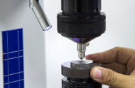
These two results are used to form a subgroup. The range between these two results is called the subgroup range and is |28.0 – 27.9| = 0.1. The range is always positive.

What does this range represent? It represents the variation in the destructive test method since the samples are the “same.” Monitoring the range values over time of duplicate samples will allow us to monitor the consistency of the destructive test method.

The resulting subgroup ranges are then plotted on a range control chart. The average range and control limits are calculated and added to the range control chart. If the range control chart is in statistical control, then the destructive test is consistent. If there are out of control points, then the destructive test is not consistent. The reasons for the out of control points should be found and eliminated.

Consistency Example

We will use hardness as the example here. Twenty subgroups of “duplicate” samples have been tested for hardness. The results are shown in Table 1 along with subgroup average and subgroup range results that we will be using in the calculations

Table 1: Hardness Duplicate Sample Results

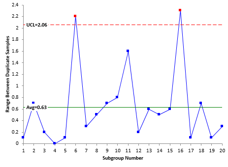
The duplicate sample results for subgroup 1 are 28.0 and 27.9. The subgroup average is 0 27.95 and the subgroup range is 0.1. The range chart for the hardness duplicate samples is shown in Figure 1.

Figure 1: Range Chart for Duplicate Samples

The range from each subgroup in Table 1 is plotted over time as shown in the figure. The average range is calculated and added to the range chart. Finally, the upper control limit (UCL) is calculated and added to the range chart. There is no lower control limit when the subgroup size is 2. Information on how the range control chart calculations are done is covered in our publication on X-R control charts.

A control chart is in statistical control if there are no points beyond the control limits and no patterns. Please see our publication on interpreting control charts if you would like more information on the various out of control tests.

Look at Figure 1. There are two subgroup ranges (subgroups 6 and 16) beyond the UCL. This means that the test method was not in statistical control for these two subgroup ranges. Something happened that caused the range between the duplicate samples to be larger for those two subgroups when compared to the rest of the subgroups. The objective is find out what happened – the special cause of variation – and prevent it from happening again. This is the only way to ensure that this destructive test method is consistent.

The objective is to remove the special causes of variation so the test method is in statistical control – no points beyond the control limits and no patterns. This is how you let your customer know that your destructive test method is consistent.

% Variance Due to Destructive Test

The basic equation describing the relationship between the total variance, the product variance and the test method variance is given below.

σ_x²= σ_p²+σ_e²

where σ_x²= total variance of the product measurements, σ_p²= the variance of the product, and σ_e²= thevariance of the measurement system.

The % variance due to the test method is then given by:

% variance due to test method = 100(σ_e^2/σ_x²)

So, to determine how much of the total variance is due to the test method, we need to determine the two sigma values in the equation above.

The measurement system variance can be determined from the average range using the following equation:

whereR is the average range, d₂ is a control chart constant that depends on the subgroup size (n). For a subgroup size of 2, the value of d₂ is 1.128.

The average range from Figure 1 is 0.63. However, this is NOT the average range you use. Remember, the range chart is not in statistical control. There are outliers – special causes of variation – present. This means that you don’t have a good estimate of the average range – and thus, cannot use the average range to find the test method variance.

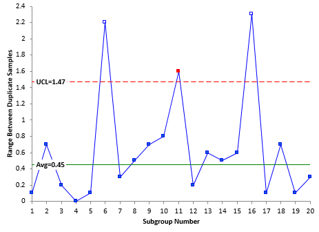
What you do at this point is remove the out of control points from the calculations. Figure 2 shows the range with subgroups 6 and 16 removed from the calculations (but still plotted on the chart). The new average range is 0.45.

Figure 2: Range Chart with Subgroups 6 and 16 Removed

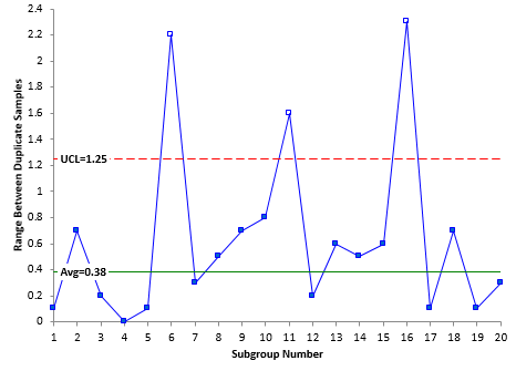
Take another look at Figure 2. Is this range chart in or out of control? There is now another point (subgroup 11) above the upper control limit – another special cause of variation. You continue to remove the out of control points until all the remaining points are in statistical control. Figure 3 shows the range chart with subgroup 11 removed.

Figure 3: Range Chart with Subgroups 6, 11, and 16 Removed

All the points are now in statistical control. The average range is 0.38 and can now be used to determine the test method variance.

This is the test method variance for the average of the duplicate samples.

You can find the total variance by constructing an individuals control chart based the subgroup averages. Note that you can’t do anX-R control chart because the ranges are based on the duplicate samples. So, you use an individuals control chart where you plot the subgroup averages from Table 1 as individual values.

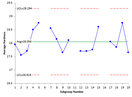
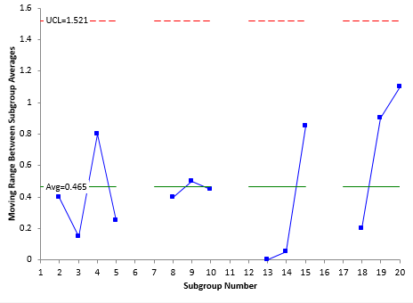
The individuals control chart is shown in figures below. Note that subgroups 6, 11 and 16 are not included since these had special causes of variation during the measurement process. The X chart is shown in Figure 4. The moving range is shown in Figure 5.

Figure 4: X Chart

Figure 5: Moving Range Chart

Figures 4 and 5 are in statistical control. This means that the production process is in statistical control. The total variance can be estimated from the average moving range. The total variance is given by:

We can now estimate the % variance due to the test method.

This tells us that the test method is responsible for 33.9% of the total variance seen in the process. This is the second piece of information your customer wanted. And since the destructive test method is consistent, this will remain true until the test method is improved. You have now answered the two findings from the audit.

You might say that 33.9% is too large for a test method. Dr. Donald Wheeler gives an excellent way of defining how good a test method is. We covered this in a previous publication. The test method is actually a second class monitor and is still very useful for monitoring the process.

Summary

This publication examined how to determine if a destructive test method is consistent. This is done by taking pairs of duplicate samples – pairs that are as much alike as possible – and using a range control chart to monitor the stability of the test method. If this range control chart is in control, then the test method is consistent. The average range can then be used to estimate the variance due to the test method. This variance can then be compared to the total process variance to determine the % of variance that is due to the test method.