December 2014
 Measurements are critical. They tells us where we are now. They tell us if we are improving performance based on past measurements – or just staying the same – or if our performance is declining. No doubt about it – we need measurements – good measurements.
So, what makes a good measurement? How do we know our measurements are “good?” Don’t we simply need to perform a Gage R&R study and find out what % of our variance is due to the measurement system? Then we simply use the AIAG recommendations – less than 10% means that the measurement system is acceptable, 10 to 30% means that the measurement system may be acceptable for some application, and greater than 30% means that the measurement system is unacceptable.
Suppose you do this for a key product characteristic. You find out that your measurement system is responsible for 44% of the total variance. What will the customer say? Should you panic? Maybe, but then again maybe not. We need to change the paradigm of how we evaluate the measurement system.
 This publication takes a look at a different method of classifying the measurement system. This procedure (developed by Dr. Donald Wheeler) divides the measurement system into four categories – First Class monitors, Second Class monitors, Third Class monitors and Fourth Class monitors.
These categories give insight into the puzzle that is our measurement system – in particularly these three characteristics of the measurement system:
- How the measurement system can reduce the strength of a signal (out of control point) on a control chart.
- The chance of the measurement system detecting a large shift.
- The ability of the measurement system to track process improvements.
These insights give you a very good understanding of the relative usefulness of the measurement system.
In this issue:
- Introduction
- Relationship between Total, Product and Measurement Variation
- Intraclass Correlation Coefficient
- Calculating the Intraclass Correlation Coefficient
- Classifying the Measurement Process
- Summary
- Quick Links
You may download a pdf version of this publication here.
Introduction
This publication challenges you to take a different look at how you define how useful a measurement system is. Much more information is available from Dr. Donald Wheeler in his book Evaluating the Measurement Process & Using Imperfect Data (available from www.spcpress.com). Definitely a book to add to your library. This procedure involves estimating the various components of variance (total, process and measurement system), much like you do when performing an ANOVA Gage R&R. The change in paradigm comes in how you interpret the results.
Relationship between Total, Product and Measurement Variation
 You take a sample from your process. You test that sample using your measurement system. You get a result (X1). You take another sample and test that sample. You get another result (X2). Usually X1 does not equal X2. What are in these results? Two major components are present in each result: the variation in the product itself and the variation in the measurement system.
The basic equation describing the relationship between the total variance, the product variance and the measurement system variance is given below.
σx2= σp2+σe2
where σx2= total variance of the product measurements, σp2= the variance of the product, and σe2= the variance of the measurement system.
We will use the ratio of the product variance to the total variance to define the “Intraclass Correlation Coefficient.” This will be used to define how useful the measurement system is. It sounds worse than it actually is.
Intraclass Correlation Coefficient
 According to Dr. Wheeler, the “Intraclass Correlation Coefficient” is the traditional measure of association used to characterize the relative usefulness of a measurement system.” When I first was introduced to this, I wondered why I had not heard this term when learning about measurement systems. You might be thinking the same thing. Well, it is the name that throw me off. Probably you too. The Intraclass Correlation Coefficient is simply the ratio of the product variance to the total variance and is denoted by ρ:
ρ= σp2/σx2
This is simply the % of the total variance that is due to product variance. Remembering the basic equation above, then 1 – ρ is the % of the total variance that is due to the measurement system. This is essentially what we look at in ANOVA Gage R&R analysis. So, you may not have heard the term “Intraclass Correlation Coefficient” but you have been exposed to the basic concept most likely.
The product variance is not easy to estimate so the value of ρ is usually rewritten to be:
ρ= σp2/σx2= (σx2-σe2)/σx2= 1 – σe2/σx2
So, to find the value of ρ, we need to estimate the total variance and the measurement system variance. Let’s take a look at one way we can do this and then determine what the value of ρ is telling us.
Calculating the Intraclass Correlation Coefficient
Suppose one of our critical to customer metrics is the viscosity of our product. We measure the viscosity four times a day. The data for the last 20 days are shown in Table 1.
Table 1: Product Viscosity Data
| Day | X1 | X2 | X3 | X4 | Day | X1 | X2 | X3 | X4 | |
|---|---|---|---|---|---|---|---|---|---|---|
| 1 | 54.6 | 56.2 | 57.8 | 56.6 | 11 | 50.7 | 51.4 | 49.0 | 52.6 | |
| 2 | 47.8 | 51.3 | 55 | 49.7 | 12 | 48.2 | 51.2 | 50.7 | 48.8 | |
| 3 | 46.6 | 50.3 | 39.3 | 45.4 | 13 | 39.5 | 39.9 | 46.4 | 39.6 | |
| 4 | 53.7 | 55.2 | 50.8 | 53.6 | 14 | 53.9 | 55.4 | 49.0 | 50.3 | |
| 5 | 53.2 | 55.4 | 55.1 | 52.2 | 15 | 52.9 | 56.1 | 53.2 | 53.0 | |
| 6 | 55.9 | 52.9 | 53.3 | 48.0 | 16 | 59.9 | 64.0 | 71.9 | 69.0 | |
| 7 | 52.5 | 53.2 | 52.2 | 49.4 | 17 | 51.8 | 57.2 | 49.2 | 56.0 | |
| 8 | 56.3 | 55.3 | 53.4 | 52.7 | 18 | 49.9 | 50.4 | 50.6 | 50.2 | |
| 9 | 61.6 | 63.3 | 55.9 | 57.1 | 19 | 59.1 | 50.3 | 52.6 | 56.7 | |
| 10 | 53.8 | 48.2 | 49.4 | 52.3 | 20 | 51 | 52.2 | 50.3 | 54.1 |
You can analyze these data using an X-R chart and then, based on the stability of the R chart, the average range can be used to estimate the total variance in product measurements. The charts are shown in Figures 1 and 2 below.
Figure 1: X Chart for Product Viscosity

Figure 2: R Chart for Product Viscosity

The X chart has some points beyond the control limits. This means that there are special causes present that created the differences in those subgroup averages. However, the R chart is in statistical control. This means we can use the average range (5.69) to estimate the total variance in the product measurements as follows:

d2 is a constant that depends on subgroup size and is equal to 2.059 for a subgroup size of 4.
So, we now have our estimate of the total variance due to the product measurements. We now need only an estimate of the total variance due to the measurement system to calculate ρ.
Suppose our lab has been testing the viscosity of a standard for the past 25 days using the measurement system. The data are shown in Table 2.
Table 2: Viscosity of Standard
| Sample | Viscosity | Sample | Viscosity | Sample | Viscosity | ||
|---|---|---|---|---|---|---|---|
| 1 | 37.6 | 10 | 42.5 | 18 | 40.9 | ||
| 2 | 38.8 | 11 | 39.2 | 19 | 36.0 | ||
| 3 | 38.3 | 12 | 39.1 | 20 | 39.1 | ||
| 4 | 37.0 | 13 | 42.0 | 21 | 40.1 | ||
| 5 | 41.2 | 14 | 39.6 | 22 | 38.0 | ||
| 6 | 41.5 | 15 | 37.2 | 23 | 40.1 | ||
| 7 | 41.0 | 16 | 42.1 | 24 | 38.5 | ||
| 8 | 38.5 | 17 | 39.7 | 25 | 39.0 | ||
| 9 | 38.8 |
We can analyze these data using an individuals control chart and, depending on the results, use the moving range to estimate the measurement system variance. Remember, this is running the same sample over and over. So, the variation in results is due to the measurement system. Figures 3 and 4 show the individuals (X) chart and the moving range chart.
Figure 3: X Chart for Repeated Viscosity Measurements for the Standard
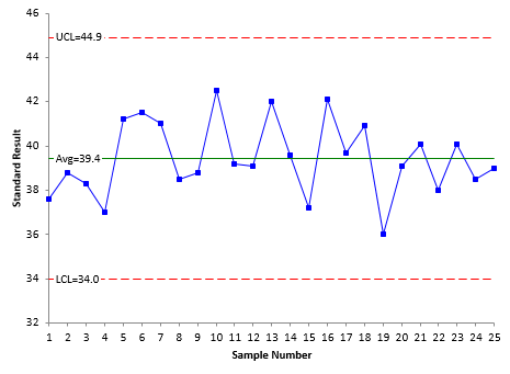
Figure 4: Moving Range Chart for Repeated Viscosity Measurements for the Standard

Both the X and moving range chart are in statistical control – there are no out of control points. The measurement system is consistent and predictable. Since the moving range chart is in control, we can estimate the measurement system variance as follows:

Now we can estimate the Intraclass Correlation Coefficient as follows:
![]()
What does this value mean? It means that, when the process is in statistical control, 56.1% of the variation in the product measurements will come from the product variation and 43.9% of the variation will be due to the measurement system.
What would the AIAG guidelines say about a measurement system that is responsible for almost 44% of the variation? It would say it is unacceptable. But look at Figure 1. This “unacceptable” measurement system was still able to detect the out of control points. It is clear we need to change our paradigm of what is “acceptable” and what is “unacceptable.” The next section takes a look at what the value of ? is telling us about the relative usefulness of the measurement system.
Classifying the Measurement Process
Dr. Wheeler uses the Intraclass Correlation Coefficient to place the measurement system into one of four classes. Table 3 (from Dr. Wheeler’s book referenced above)summarizes these classes and the characteristics of those classes.
Table 3: The Four Classes of Process Monitors
| Intraclass coefficient | Type of Monitor | Reduction of Process Signal | Chance of Detecting ± 3 Std. Error Shift | Ability to Track Process Improvements |
|---|---|---|---|---|
| 0.8 to 1.0 | First Class | Less than 10% | More than 99% with Rule 1 | Up to Cp80 |
| 0.5 to 0.8 | Second Class | From 10% to 30% | More than 88% with Rule 1 | Up to Cp50 |
| 0.2 to 0.5 | Third Class | From 30% to 55% | More than 91% with Rules 1, 2, 3 and 4 | Up to Cp20 |
| 0.0 to 0.2 | Fourth Class | More than 55% | Rapidly Vanishing | Unable to Track |
 The first column lists the value of the Intraclass Correlation Coefficient. The second column lists whether it is a First Class, Second Class, Third Class or Fourth Class monitor – with “First” being the best. In the viscosity example above, ρ = 0.561, so the viscosity measurement system is classified as a “Second Class” monitor. Remember that the % of the variance due to the measurement system is 1 – ρ. So, as you move from a First Class to a Fourth Class monitor the % of variance due to the measurement system is increasing.
The third column shows how much of a reduction in a process signal there is. The First Class monitor has less than a 10% reduction in process signal while a Fourth Class monitor has more than a 55% reduction in process signal. The viscosity measurement system is a Second Class monitor which has a 10 to 30% reduction in signal. Even so, it was still able to pick up the out of control points shown in Figure 1.
The fourth column lists the chance of detecting a ± 3 standard error shift within ten subgroups. This column refers to four rules. These are the four Western Electric zone tests:
-
Rule 1: a point is beyond the lower or upper control limit
-
Rule 2: two out of three consecutive points on the same side of the average are more than two standard deviations away from the average
-
Rule 3: four out of five consecutive points on the same side of the average are more than one standard deviation away from the average
-
Rule 4: Eight consecutive points are above or below the average
The “standard deviation” in the Western Electric rules is the standard deviation of what is being plotted and can be found by dividing the upper part of the control chart into three equal zones and the bottom part of the chart into three equal zones. For more information, please see our publication on how to interpret control charts. Note that the First and Second Class monitors detect Rule 1 very well. Once you reach a Third Class monitor, you need to apply all four rules to get the chance of detecting the shift high. Fourth Class monitors are not good at detecting any shifts essentially.
 The fifth column describes the monitor’s ability to track process improvements. This is something we don’t think about too much. Suppose you make a great process improvement. Your Six Sigma team worked hard and reduced the variation in the process considerably – resulting in a great improvement in your process capability value. What happened to your measurement system? Assuming you did not improve it, the % variance due to the measurement system increased as you made other improvements. This last column describes how much process improvement you can have until the measurement system moves from one class to another.
One value of process capability is the Cp value where:
![]()
where USL = the upper specification limit and LSL = lower specification limit. The equation for the Intraclass Correlation Coefficient can be rearranged as follows:
![]()
Thus, Cp can be rewritten as:

This equation can be used to generate the following value for Cp80 for a First Class monitor:

If you reduce your process variation to point where the process capability is larger than Cp80, then the Intraclass Correlation Coefficient becomes less than 0.8 and the measurement system is no longer a First Class monitor. The values of Cp50 (for a Second Class monitor) and Cp20 (for a Third Class monitor) are calculated similarly:

The viscosity measurement system, our example, is a Second Class monitor. Suppose our product has the following specifications: USL = 65 and LSL = 45. We know that σx= 2.76 from our R chart on the product measurements (Figure 2 above). Our value of Cp is then:
![]()
 As a Second Class monitor, it can track process improvements up to Cp50. We know σe= 1.83 from the moving chart on the standard (Figure 4 above). Thus:

This means that if you reduce process variation to a point where your Cp = 1.29, the measurement system will move from a Second Class to a Third Class monitor. In fact, the value of Cp20 represents the maximum process improvement you can track with the current measurement system. In this case:

This is the maximum process improvement that the measurement system will be able to track. At this point, it becomes a Fourth Class monitor and is pretty much worthless for tracking process improvements. You will need a new measurement system at this point.
This is the type of insight this method of classifying measurement systems provides. The process is not more difficult than a basic Gage R&R study – in fact, you should already be maintaining a control chart on your production process for critical to customer metrics – and running a standard on a regular basis to monitor the test methods for those critical metrics. If you are you doing this, you already have the data you need to classify these critical measurement systems.
Summary
This publication examined a different method of classifying the measurement system. This procedure divides the measurement system into four categories – first class monitors, second class monitors, third class monitor and fourth class monitors. These categories give insight into three characteristics of the measurement system:
-
How the measurement system can reduce the strength of a signal (out of control point) in a control chart.
-
The chance of the measurement system detecting a large shift.
-
The ability of the measurement system to track process improvements.
These insights give you a very good understanding of the relative utility of the measurement system. This method provides much more insight into the measurement system than the classical Gage R&R approach – even if you are using the ANOVA approach (as you should over the Average and Range method for Gage R&R). We will continue taking a look at how to evaluate the measurement process next month.
Спасибо за подробное объяснение проблемы, которые, как правило, обошел в методах использования контрольных карт Шухарта.
I tried to translate this using Google: this is what it said “Thanks for the detailed explanation of the problem, which is usually walked in the way of using Shewhart control charts.” Thanks for the feedback.
Thanks to all of you who are responsible for creating this particular outlook on this area. Initially, I thought that using control charts would help me apply a solid and different perspective to the challenge of educating myself and others about estimating measurement uncertainty. As I dove into the resources you have provided I have been suprised to find as much controversy as any other topic in applied statistics. I guess that I assumed that this area was all well settled because it was a topic on the ASQ Quality Engineer exam and because it has been discussed for such a long period! I appreciate your non-confrontational, non-troll approach to educating others about the topics here. Please keep it up!
Both Parts 1 and 2 were outstanding. You make a tremedously difficult topic very, very understandable and useful!Jeff
Howdy, You echo Wheeler's concern about overspecifying the gage requirements using the standard AIAG manual. Also, I noticed that you take a similar stance about a gage with "32%" may be just fine for a test step. The Intraclass Correlation is a truly classical metric and I think it offers a better first appproach to simply answer if the gage is ok or not — then ANOVA or something else can be used for iddentification of the issues. Wheeler posed his 4 classes, and he's also done a lot of work on this. I also had basically dropped the AIAG except when the test spec required the high precision. And I have revamped GRR completely for internal purposes. Now, for the question: It has been several years since all this came out. MSA 4th Ed did not adopt any changes. Is AIAG looking at a new edition of the MSA which will include a robust treatment of the ICC, as well as numerous other changes that I (and I think you, others and Wheeler) think should be done?Thanks
Hello. Thanks for the comment. I am not aware that AIAG is doing anything to update their information. I believe they need to.