Probable Error and Your Measurement System

April 2016

(Note: all the previous SPC Knowledge Base in the measurement systems analysis category are listed on the right-hand side. Select this link for information on the SPC for Excel software.)

Probable error. Not a term you hear too often with respect to your measurement systems. You hear things like repeatability, precision, reproducibility, %GRR. But Probable Error? What is Probable Error? Yes, it has to do with measurement error. 50% is in there somewhere. Is Probable Error of any use to you? Yes, it is.

You take measurements on a process. Maybe your measurements are in increments of 0.01. Is that measurement increment adequate? Is it too small? Why not take measurements in increments of 0.1? The Probable Error helps you determine what size your measurement increment should be.

This month’s publication is designed to help you understand probable error and how it impacts your measurement system. It really defines how precise your measurement system can be – and defines a range of effective increments for your measurement system. Of course, control charts play a role. And Probable Error helps you set your manufacturing specifications – a topic for next month.

In this issue:

• Measurement System Precision
• Measurement System Standard Deviation – What Does It Mean?
• Probable Error Definition
• Using the Probable Error
• Example
• Summary
• Quick Links

Please feel free to leave a comment at the end of the publication. You can also download a pdf copy of this publication at this link.

Measurement System Precision

Most of the time, the precision of a measurement system is reported as an estimated standard deviation. This is easily found by using repeated measurements on the same sample performed by the same operator– and using a control chart to ensure that the results are consistent. Suppose one operator measures the same sample 20 times. The results are given in Table 1.

Table 1: Repeated Measurements of Same Sample

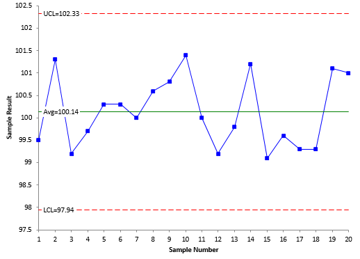
Note that the measurement increment in Table 1 is 0.1. The results in Table 1 were analyzed using an individuals control chart. The X chart is shown in Figure 1.

Figure 1: X Control Chart for Repeated Measurements of Same Sample

Each individual result is plotted on the X control chart. The purpose of this control chart is to determine if the results are consistent. As long as there are no out of control points, the measurement process is consistent with respect to the average. There are no out of control points, so the X control chart is consistent (in statistical control).

Figure 2 is the moving range chart for the data in Table 1. The moving range chart plots the moving range between consecutive results. There are two purposes to this control chart. One is to determine if the moving range between consecutive results is consistent over time. As long as there are no out of control points, the moving range is consistent (in statistical control). This is true for the control chart in Figure 2.

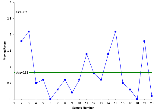
Figure 2: Moving Range Chart for Repeated Measurements of the Same Sample

The other purpose is to estimate the standard deviation of the measurement system. You can do this as long as the moving range control chart is in statistical control. Note that it does not matter if the X control chart is in control or not. The standard deviation for the measurement system (σ_ms) is given by:

σ_ms=R/1.128

The 1.128 value applies only to individuals control charts.

The average range from Figure 2 is 0.83, so σ_ms is given by:

σ_ms=R/1.128 =0.83/1.128=0.74

Measurement System Standard Deviation – What Does It Mean?

What does the standard deviation we just calculated mean? What is it estimating? A standard deviation is a measure of the variation in individual results. In this case, it is measuring the variation in repeated measurements on the same sample.

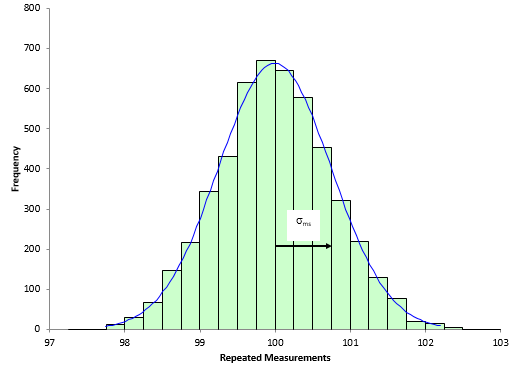
Suppose instead of 20 times, we measured the same sample 5000 times. Wow. Lots of times. To simulate this, 5000 random numbers were generated from a normal distribution population with an average of 100 and a standard deviation of 0.75. The resulting histogram is shown in Figure 3.

Figure 3: Repeated Measurements Histogram

A normal curve has been superimposed on the histogram. So, what does σ_ms mean on this chart? The arrow on the figure depicts the distance from the average (100) to 1 standard deviation above the average (100.75). For a normal distribution, the % of results that fall between the average and 1 standard deviation above the average is about 34%. This means that 34% of the repeated measurements fall between 100 and 100.75. Likewise, about 34% of the repeated measurements fall between the average and one standard deviation below the average (99.25).

The following is true for a normal distribution:

• About 68% of the values fall between -1 and +1 standard deviation from the average
• About 95% of the values fall between -2 and +2 standard deviations from the average
• About 99.97% of the value fall between -3 and +3 standard deviations from the average

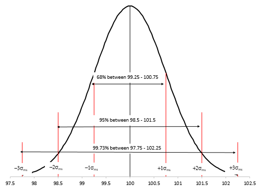
If the “true” average of the sample is 100 and the “true” standard deviation is 0.75, then 68% of the time the repeated measurement will be between 99.25 and 100.75. 95% of the time the repeated measurement will be between 98.50 and 101.50. And 99.97% of the time, the repeated measurement will be between 97.75 and 102.25. This is shown in Figure 4.

Figure 4: Repeated Measurements Normal Distribution

Probable Error Definition

Probable Error provides another method of describing the measurement variation. Dr. Donald Wheeler’s book, EMP III Evaluating the Measurement Process (www.spcpress.com), contains information on using the Probable Error. This book was used as a reference for the material below.

The Probable Error (PE) is defined as the following:

PE = 0.675σ_ms

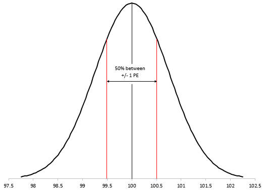
What is special about the value of PE? The PE defines the middle 50% of the normal distribution as shown in Figure 5.

Figure 5: Probable Error

This means that half of the repeated measurements should fall between the average and ± PE as shown below:

X ± 1 PE

X ± 0.675σ_ms

100 ± 0.675(0.75)

100 ± 0.50625

Thus, 50% of the repeated measurements lie between 99.494 and 100.506.

Using the Probable Error

What does this mean for your measurement process? Obviously, it means that 50% of the time the result will within one PE of the average – and 50% of the time it will be outside 1 PE. OK, so what? This actually places limits on the resolution of your measurement system – and the PE can be used to help determine the measurement increment. In Dr. Wheeler’s words:

“No measurement should ever be interpreted as being more precise than plus or minus one Probable Error since your measurement will err by this amount or more at least half the time.”

You can use the PE to determine how many digits you should record your test results at. The goal is to have the measurement increment about the same size of the PE. Dr. Wheeler gives the following guidelines for determining a range of effective measurement increments:

Smallest Effective Measurement Increment = 0.2PE

Largest Effective Measurement Increment = 2PE

Look at the data in Table 1. The measurement increment is 0.1. The PE from above is 0.50625. Thus:

Smallest Effective Measurement Increment = 0.2PE = .2(.50625) = .10125

Largest Effective Measurement Increment = 2PE = 2(.50625) = 1.0125

The measurement increment of 0.1 may be too small in this case as it is just about equal to the smallest effective measurement increment. When the measurement increment is too small, the measurement looks better than it really is. In this case, you need to increase the measurement increment so it is between 0.2PE and 2PE. If the measurement increment is too large, you will need to decrease the measurement increment so it is within the range. Let’s look at another example.

Example

Ten parts are pulled from a process and measured three times each by one operator. The data are shown in Table 2.

Table 2: Product Data

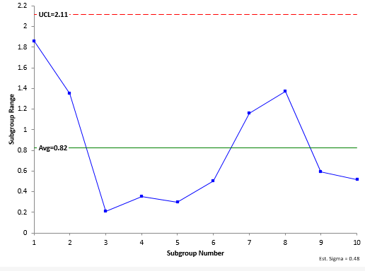
Note that the measurement increment is 0.01. These data can be analyzed using an X-R chart. Here we will only be concerned with the R chart. The R chart is shown in Figure 6.

Figure 6: R Chart for Product Data

The range chart is measuring the variation in the measurement system since the within subgroup variation represents measurements on the same part. It is in statistical control. Thus, we can estimate the measurement system standard deviation as follows:

σ_ms=R/d₂ =0.82/1.693=0.48

d₂ is a control chart constant that depends on subgroup size (n = 3 in this example). The Probable Error is then given by:

PE = 0.675(σ_ms) = 0.675(0.48) = 0.324

Note that the PE is equal to 32 times the measurement increment. The measurement increment is too small. The range of effective measurement increments is from 0.2PE to 2PE or 0.0648 to 0.648. Thus, the 0.01 digit is not meaningful. The measurement increment should be increased to 0.1

Summary

The standard deviation of a measurement system is used most often to report the precision. This publication reviewed what this standard deviation means. Then, we took a look at the Probable Error of a measurement system. A single repeated measurement on the same sample with fall within 1 Probable Error of the average 50% of the time. This Probable Error is used to help define the range of effective measurement increments. If the measurement increment falls outside the range, the measurement increment needs to be increased or decreased. Probable error also plays an important role in setting manufacturing specifications as we will see next month.