October 2007
In This Issue:
This newsletter is the second in a series on variable measurement systems and how to understand the impact these measurement systems have on your operations. Measurement systems are extremely important in continuous process improvement. We must measure to know where we are. We use measurements to tell us if there is a problem in the process or if a process change has improved the process.
For measurements to be effective, they must be timely, accurate, and precise. Many of our customers, both internal and external, rely on our measurements. So how do we provide measurements that are meaningful? That is the purpose of this series of newsletters. Last month, we covered stability of measurement systems. This month we examine bias in measurement systems.
Bias Definition
The third edition of the book Measurement Systems Analysis (published by AIAG) has the following definition for bias:
“Bias is the difference between the true value (reference value) and the observed average of the measurements on the same characteristic on the same part.”
Bias is sometimes called accuracy. Accuracy (and bias) refers to the absolute correctness of the measurement system relative to a standard. There are many standards. For example, one method of checking the accuracy of a laboratory weigh scale is to put a standard 10 gram weight on the scale. On average, the scale should read 10 grams if it is accurate.
Another example involves an on-line gas analyzer. To check the accuracy of this analyzer, a standard gas is injected into the analyzer. On average, the analyzer should indicate the standard gas composition if the analyzer is accurate. Obviously, we want measurement systems that reflect the true value of a standard.
Bias represents a measure of the systematic error of a measurement system. The AIAG book lists some reasons for excessive bias including:
- Instrument needs recalibrating
- Worn equipment
- Damaged master
- Improper calibration
- Temperature
- Humidity
- Cleanliness
The process for conducting a study to determine if there is bias in a measurement system is given below. It is important that the measurement system be stable (in statistical control) when the bias study is done. This is done by running a standard on a regular basis, plotting the results on a control chart and interpreting the results for statistical control. How to do this was covered in last month’s newsletter.
Independent Sample Method
The steps in conducting a bias study for a measurement system are given below. To perform a bias study, you must have a reference with a known value.
- Determine the reference value.
- You would like to compare your measurement system to a traceable standard. For example, scales often have weights that serve as standards. In this case, obtain a sample and determine its reference value relative to the traceable standard.
- Run the sample at least 10 times using one appraiser and the measurement system in the normal manner and record the results. The more times you run the sample the greater the accuracy of the bias study.
Analyzing the Results
The results can be analyzed in two ways:
- Graphically using a histogram
- Numerically by developing a confidence interval around the average and determining if the interval contains zero
To see how to analyze the results, we will use the following example:
A hardness tester is used to test steel for Rockwell hardness. The lab supervisor wants to determine if the tester has any bias. He has a standard block that has a hardness of 36. This block is supplied by the vendor and it is traceable back to a standard. The lab supervisor decides to have one lab technician run the block 15 times in the hardness tester. The results are shown below.
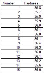
The lab supervisor will use these results to determine if the hardness tester has any bias. The first step is to make a histogram of the results. This histogram is shown below.
The histogram shows that the hardness results are spread out around the reference value. This indicates that there is no bias present.
To further assure that there is no bias present, the lab supervisor constructs a 95% confidence interval around the average hardness result. If the confidence interval includes 36, the reference value, the lab supervisor will assume there is no evidence of bias being present.
The steps in constructing this confidence interval are given below.
- Determine the average of the n = 15 hardness results (Xbar = 36.00667)
- Determine the bias = Xbar – reference value (bias = 0.00667)
- Determine the standard deviation (s = 0.21202)
- Determine the degrees of freedom (df = n-1 = 14)
- Determine the alpha level (confidence coefficient) you want (alpha = 0.05)
- Find the t value for the t distribution for df and alpha (t = 2.144787)
- Calculate the upper confidence limit:
- Upper confidence limit = Xbar + t*s/sqrt(n) = 36.12408
- Calculate the lower confidence limit:
- Lower confidence limit = Xbar – t*s/sqrt(n) = 35.88925
Since the confidence limit contains 36, the lab supervisor concludes that there is no evidence of bias. t values are available in many statistics books and in Excel using the TINV function.
Bias Example
A colorimeter is used to measure the color of a powder. A white sample has a color of 100 and is traceable to a standard. A lab technician ran the sample ten times and recorded the color. The results are given below.
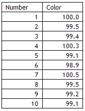
A histogram based on these results is shown below. The results do include 100 but there appear to be more results to the left of 100 than to the right.
The confidence interval around the average is constructed as shown below.
- Determine the average of the n = 10 color results (Xbar = 99.55)
- Determine the bias = Xbar – reference value (bias = -0.45)
- Determine the standard deviation (s = 0.542115)
- Determine the degrees of freedom (df = n-1 = 9)
- Determine the alpha level (confidence coefficient) you want (alpha = 0.05)
- Find the t value for the t distribution for df and alpha (t = 2.262157)
- Calculate the upper confidence limit:
- Upper confidence limit = Xbar – t*s/sqrt(n) = 99.93781
- Calculate the lower confidence limit:
- Lower confidence limit = Xbar – t*s/sqrt(n) = 99.16219
The confidence limit ranges from 99.16 to 99.94. This range does not include 100. So, it appears that there is bias in the measurement system that must be addressed.
Summary
Last month, we started our analysis of variable measurement systems. The first step in analyzing the performance of a measurement system is to ensure it is stable, i.e., in a state of statistical control. This is determined by finding a master sample, measuring it over time, and plotting the results on a X-mR chart. The X-mR chart is then analyzed for statistical control. It there are out-of-control points present, the causes of these must be eliminated. Once there are no out-of-control points, the measurement system is stable and further analysis can be done. The next step is to ensure that there is no bias in the measurement. In this newsletter, an independent sample method was introduced to accomplish this.
Next month we will continue our examination of measurement systems and examine linearity.