- Linearity Definition
- Linearity Study
- Analyzing the Results
- Interpreting the Results
- Summary
- Quick Links
This newsletter is the third in a series on variable measurement systems and how to understand the impact these measurement systems have on your operations. Measurement systems are extremely important in continuous process improvement. We must measure to know where we are. We use measurements to tell us if there is a problem in the process or if a process change has improved the process.
For measurements to be effective, they must be timely, accurate, and precise. Many of our customers, both internal and external, rely on our measurements. So how do we provide measurements that are meaningful? That is the purpose of this series of newsletters.
The first series covered stability of measurement systems and how to use control charts to monitor the stability of measurement systems. In the last series we examined bias in measurement systems. Bias occurs when there is a difference between the true value (reference value) and the observed average of the measurements on the same characteristic on the same sample. In this newsletter we examine linearity of measurement systems. Linearity is concerned with the bias throughout the measurement range.
Linearity Definition
The third edition of the book Measurement Systems Analysis (published by AIAG) has the following definition for linearity:
“The difference of bias throughout the expected operating (measurement) range of the equipment is called linearity.”
This means that you cannot assume constant bias throughout the measurement range. Possible causes of linearity issues include:
- Measurement system needs calibration
- Poor maintenance on the measurement system
- Problem with the master
- Temperature
- Humidity
- Cleanliness
- Poor measurement system design
The process for conducting a study to determine if there is linearity in a measurement system is given below. It is important that the measurement system be stable (in statistical control) when the linearity study is done. This is done by running a standard on a regular basis, plotting the results on a control chart and interpreting the results for statistical control. How to do this was covered in the first series on measurement systems analysis.
Linearity Study
The steps in a linearity study are given below. The key starting point is selecting samples to include in the study. These samples must span the range of the measurement variation in the process. For example, if your process output varies from 70 to 100, you want to select samples that span that range. You don’t want to only include samples in the 90 to 100 range. You linearity study will not be valid for the entire range. It is best to have at least 5 samples over the range.
Another problem is determining the reference value for the samples. This can be done, for example, if you have a master toolroom. You may have to send out the samples to another lab which you know has better precision than your lab.
The last issue is to be sure that one operator measures each sample at least 10 times. The samples should be measured in a random order.
Thus, the steps in conducting a linearity study are:
- Select at least 5 samples the measurement values of which cover the range of variation in the process
- Determine the reference value for each sample
- Have one operator measure each sample at least 10 times using the measurement system
Analyzing the Results
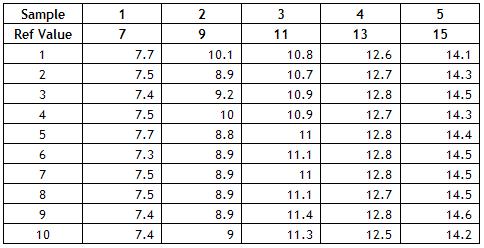
To show how to analyze the results, we will use the following example. A lab supervisor wants to check the linearity of a new measurement system. He collects five samples over the range of production and determines the reference value for each sample. He then has one operator run each sample 10 times in a random order. The results are given below.
To analyze the results, follow the steps below.
Calculate the bias for each measurement. This is done by subtracting the reference value from the measurement result. For example, the measurement result for the first measurement for the first sample was 7.7. The bias is then 7.7 – 7 = 0.7. The bias for all measurements is shown in the table below.
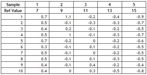
Calculate the average bias for each sample. This is done by adding up the bias results for each sample and dividing by the number of times each sample was tested. For example, for sample 1, the sum of the bias results is 4.9. Since the sample was tested 10 times, the average bias for sample 1 is 4.9/10 = 0.49. The averages for all samples are shown below.
- Sample 1: 0.49
- Sample 2: 0.16
- Sample 3: 0.02
- Sample 4: -0.28
- Sample 5: -0.61
Plot the individual bias results and the average bias versus the reference value for each sample. The plot is shown below.
- Determine the best fit line for the average bias results and add it to the chart.
- The best fit line is given by ybar = b1x + b0 where ybar = bias average and x = reference value for each sample.
The easiest way to do this is to use Microsoft Excel. You can easily add the trend line by right-clicking on the chart and selecting “Add Trendline.” You can also select the option to add the equation for the best fit line. This equation is ybar = -0.132x + 1.408.
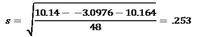
Determine the standard deviation (s) using the following equation:
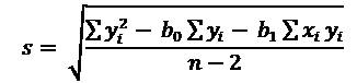
where n = total number of measurements (number of samples * number of repeat measurements = 5 * 10 = 50), yi is the individual bias results and xi is the reference value. Thus,
Determine the 95% upper confidence band (UCB) and lower confidence band (LCB) for each value of x0:

where t(0.05, df) is the value for the t distribution for n – 2 degrees of freedom nd 95% confidence. This is available from Microsoft Excel using the TINV function. For 48 degrees of freedom, the value of t is 2.011. The calculations for each value of the confidence band are not shown here.
Plot the confidence bands and the bias = 0 line on the chart. The final chart is shown below.
Interpreting the Results
The results can be interpreted graphically and numerically. If linearity is acceptable, the bias = 0 line must fall entirely within the confidence bands. This is clearly not the case in the above chart. So, there appears to be a problem with linearity.
You can also analyze the results numerically. The question you want to answer is “Is the slope of the bias line significantly different from 0?” To do this, you calculate the following t value:

The denominator is the reference value xi minus the average reference value. The value of t for this data is 10.433. You compare this value of t to the critical t value for 48 degrees of freedom and 95% confidence. As shown above, the critical value of t is 2.011. If the absolute value of the calculated t value is greater than the critical value of t, then the slope is significantly different than zero. Since 10.433 is greater than 2.011, we conclude that the slope of the bias line is not 0 and that the linearity is not acceptable. This issue must be addressed and corrected before the measurement system can be used.
Summary
In the first series, we started our analysis of variable measurement systems. The first step in analyzing the performance of a measurement system is to ensure it is stable, i.e., in a state of statistical control. This is determined by finding a master sample, measuring it over time, and plotting the results on a X-mR chart. The X-mR chart is then analyzed for statistical control. It there are out-of-control points present, the causes of these must be eliminated. Once there are no out-of-control points, the measurement system is stable and further analysis can be done.
The next step is to ensure that there is no bias in the measurement. In the second series, an independent sample method was introduced to accomplish this. In this newsletter, we examined linearity to ensure that there is no bias over the range of measurements expected.
Next month we will continue our examination of measurement systems and examine gage R&R. This permits us to determine how acceptable the measurement system is.