December 2007
In This Issue:
- Definitions
- Planning the Gage R&R Study
- Analyzing the Results
- Interpreting the Results
- Summary
- Quick Links
Note to our readers: this publication discusses the average and range Gage R&R methodology. It is still used today by some, but more accurate information is gained by using the Evaluating the Measurement Process developed by Dr. Donald Wheeler or the ANOVA method. More information on these techniques can be found in the list on the right-hand side of this page.
This newsletter is the fourth in a series on variable measurement systems and how to understand the impact these measurement systems have on your operations. Measurement systems are extremely important in continuous process improvement. We must measure to know where we are. We use measurements to tell us if there is a problem in the process or if a process change has improved the process.
For measurements to be effective, they must be timely, accurate, and precise. Many of our customers, both internal and external, rely on our measurements. So how do we provide measurements that are meaningful? That is the purpose of this series of newsletters.
The first newsletter in the series covered stability of measurement systems and how to use control charts to monitor the stability of measurement systems. If the measurement system is not in statistical control, you can never be sure of the results you are obtaining.
We then examined bias in measurement systems. Bias occurs when there is a difference between the true value (reference value) and the observed average of the measurements on the same characteristic on the same sample. In the third newsletter, we examined linearity of measurement systems. Linearity is concerned with the bias throughout the measurement range.
In this newsletter we will take a look at the statistical tool called gage repeatability and reproducibility or Gage R&R for short. This tool measures the amount of variation in the measurement system arising from the measurement device and the people taking the measurements. This newsletter covers the average and range method for analyzing the results of a Gage R&R.
Definitions
 We will use the term “gage” to refer to the measurement device in this newsletter. A gage R&R study usually is performed using 2 to 3 appraisers and 5 to 10 parts. Each appraiser measures the parts multiple times. Two components are being examined: gage variation (repeatability) and appraiser variation (reproducibility).
Repeatability is the “within appraiser” variation. It measures the variation one appraiser has when measuring the same part (and the same characteristic) using the same gage more than one time. This variation is usually referred to as Equipment Variation (EV) in the gage R&R study. This is also called the “within system” variation.
Reproducibility is the “between appraisers” variation. It is the variation in the average of the measurements made by the different appraisers when measuring the same characteristic on the same part. This is also called the “between system” variation.
Planning the Gage R&R Study
The basic steps in planning a gage R&R study are given below.
1. Determine the number of parts, the number of appraisers to use and the number of trials. 
There are several issues that must be considered when planning a gage R&R study. The first is the number of appraisers and the number of parts to use. The number of parts (n) must be greater than or equal to 5. The number of appraisers (k) must be greater than 2. The number of trials (r) must be greater than or equal to two. This represents how often each appraiser will measure a part.
In addition, the n*k should be greater than 15. This gives more confidence in the results. If possible, include all the appraisers who operate the gage in the study.
2. Select the parts for the study
The next step is selecting the parts to include in the study. There are three ways to determine the % gage R&R. One is to compare the gage variation to the variation of the parts used in the study. In this case, the parts should be selected to reflect the range of variation in the process. In other words, don’t just take 10 parts off the line right in a row. You need to select the parts so they reflect the variation seen in the manufacturing process.
The other two ways to determine the % gage R&R is to use an independent estimate of the process variation or to compare the results to the specification range. If you have an independent estimate of the process variation (e.g., from a control chart kept on the production process), the requirement for the parts spanning the production range is less critical. This is also true if you are comparing the results to the specification range.
3. Label the parts from 1 to n and designate the appraisers A, B, etc.
4. Conduct the Measurements
The parts must be run in random order. Start with appraiser A. Appraiser A measures the parts in random order. The results are recorded. This process continues for each appraiser without the appraisers being able to see the results from other appraisers. This cycle is continued until you have completed all trials. Be sure that an appraiser cannot see his/her results from previous trials.
Analyzing the Results
To demonstrate how to analyze the results, we will use the following example. Suppose you want to determine if a certain gage is capable of measuring the length of a certain part. You decide to do a basic gage R&R study. You select three appraisers (A, B, and C). You select five parts that represent typical variation in the length output. You have each appraiser measure each part three times. The measurement results are given below.
| App | Trial | Part 1 | Part 2 | Part 3 | Part 4 | Part 5 |
| A | 1 | 3.29 | 2.44 | 4.34 | 3.47 | 2.20 |
| A | 2 | 3.41 | 2.32 | 4.17 | 3.50 | 2.08 |
| A | 3 | 3.64 | 2.42 | 4.27 | 3.64 | 2.16 |
| B | 1 | 3.08 | 2.53 | 4.19 | 3.01 | 2.44 |
| B | 2 | 3.25 | 1.78 | 3.94 | 4.03 | 1.80 |
| B | 3 | 3.07 | 2.32 | 4.34 | 3.20 | 1.72 |
| C | 1 | 3.04 | 1.62 | 3.88 | 3.14 | 1.54 |
| C | 2 | 2.89 | 1.87 | 4.09 | 3.20 | 1.93 |
| C | 3 | 2.85 | 2.04 | 3.67 | 3.11 | 1.55 |
You use the above results to perform the gage R&R calculations. You start by determining the following:
- The average for each trial for each appraiser
- The average and range for each part for each appraiser
- The overall average and average range for each appraiser
- The overall average and the average range for the part
These calculations are shown in the table below.
| Appraiser | Trial/Part | 1 | 2 | 3 | 4 | 5 | Average |
| A | 1 | 3.29 | 2.44 | 4.34 | 3.47 | 2.20 | 3.148 |
| A | 2 | 3.41 | 2.32 | 4.17 | 3.50 | 2.08 | 3.096 |
| A | 3 | 3.64 | 2.42 | 4.27 | 3.64 | 2.16 | 3.226 |
| A Average | 3.45 | 2.39 | 4.26 | 3.54 | 2.15 | 3.157 | |
| A Range | 0.35 | 0.12 | 0.17 | 0.17 | 0.12 | 0.186 | |
| B | 1 | 3.08 | 2.53 | 4.19 | 3.01 | 2.44 | 3.050 |
| B | 2 | 3.25 | 1.78 | 3.94 | 4.03 | 1.80 | 2.960 |
| B | 3 | 3.07 | 2.32 | 4.34 | 3.20 | 1.72 | 2.930 |
| B Average | 3.13 | 2.21 | 4.16 | 3.41 | 1.99 | 2.980 | |
| B Range | 0.18 | 0.75 | 0.40 | 1.02 | 0.72 | 0.614 | |
| C | 1 | 3.04 | 1.62 | 3.88 | 3.14 | 1.54 | 2.644 |
| C | 2 | 2.89 | 1.87 | 4.09 | 3.20 | 1.93 | 2.796 |
| C | 3 | 2.85 | 2.04 | 3.67 | 3.11 | 1.55 | 2.644 |
| C Average | 2.93 | 1.84 | 3.88 | 3.15 | 1.67 | 2.695 | |
| C Range | 0.19 | 0.42 | 0.42 | 0.09 | 0.39 | 0.302 | |
| Part Average | 3.17 | 2.15 | 4.10 | 3.37 | 1.94 | 2.944 | |
| Part Range | 0.79 | 0.91 | 0.67 | 1.02 | 0.90 | 0.858 |
You then determine the average range for the three appraisers.
Then determine the difference between the maximum appraiser average and the minimum appraiser average. A has the maximum average (3.157). C has the minimum average (2.695).
![]()
Thus, the difference is 3.157 – 2.695 = 0.462.
Next determine the range of the part averages (Rp). The largest part average is for Part 3 (4.099). The smallest part average is for Part 5 (1.936).
![]()
So, Rp = 4.099 – 1.936 = 2.163
The various contributors to the measurement system variation can now be calculated. There are five that need to be calculated:
- Equipment variation (EV)
- Appraiser variation (AV)
- Repeatability and reproducibility (GRR)
- Part variation (PV)
- Total variation (TV)
Repeatability: Equipment Variation (EV)
This is the “within appraiser” variation. It measures the variation one appraiser has when measuring the same part (and the same characteristic) using the same gage more than one time. The calculation is given below.
![]()
where K1 is a constant that depends on the number of trials. For 2 trials, K1 is 0.8862. For 3 trials, K1 is 0.5908. For this example:
![]()
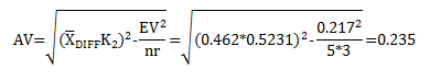
Reproducibility: Appraiser Variation (AV)
This is the “between appraisers” variation. It is the variation in the average of the measurements made by the different appraisers when measuring the same characteristic on the same part. The calculation is given below.
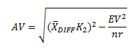
where K2 is a constant that depends on the number of appraisers. For 2 appraisers, K2 is 0.7071. For three appraisers, K2 is 0.5231 For this example:
Repeatability and Reproducibility (GRR)
The next calculation combines the two above to determine GRR, which is given by:
![]()
For this example,
![]()
Part Variation (PV)
The part variation is determined by multiplying the range of the part averages (Rp) by a constant K3. K3 depends on the number of parts. For 5 parts, K3 = 0.4030. The part variation is then given by:
![]()
Below are some other values of K3 for different numbers of parts:
| Parts |
K3 |
| 2 | 0.7071 |
| 3 | 0.5231 |
| 4 | 0.4467 |
| 5 | 0.4030 |
| 6 | 0.3742 |
| 7 | 0.3534 |
| 8 | 0.3375 |
| 9 | 0.3249 |
| 10 | 0.3146 |
Total Variation (TV)
This is the total variation from the study. It is determined by the following equation:
![]()
Interpreting the Results
Remember, a gage R&R study is a study in variation. You must have variation in the parts and in the appraisers to calculate the above numbers. To determine if the measurement system is adequate, you must compare the results to something.
If you want to compare the results to the variation in the parts used in the study, you use the total variation (TV). Then you do the following calculations:
%EV = 100(EV/TV) = 100(0.217/0.9285) = 23.3%
% AV = 100(AV/TV) = 100(0.235/0.9285) = 25.3%
%GRR = 100(GRR/TV) = 100(0.319/0.9285) = 34.3%
%PV = 100(PV/TV) = 100(0.872/0.9285) = 93.9%
Don’t expect these percentages to sum to 100 because they will not. The number that most people focus on first is the % GRR. The following guidelines can be used to determine if the measurement system is acceptable:
- % GRR under 10% of TV: Measurement system is acceptable
- % GRR from 10% to 30% of TV: Measurement system may be acceptable based on the application
- % GRR over 30% of TV: Measurement system needs improvement
In this example, the measurement system needs improvement since %GRR is greater than 30%. Sometimes you can look at the %AV and %EV to get insights into where to start improving the measurement system. But the study indicates that the measurement system must be improved.
If you want to compare the results to the tolerance instead of the total variation, you would substitute the (USL – LSL)/6 for TV.
You can also determine the number of distinct categories (ndc). This is a measure of the number of distinct categories that can be distinguished by the measurement system. It is similar to looking at how many possible values there are on a range control chart. The calculation is:
ndc = 1.41(PV/GRR) = 1.41(0.872/0.319) = 3.8
The integer value of ndc should be greater than or equal to 5. In this case, it is 3. Again, this is an indication that the measurement system needs improvement.
Summary
 In the first series, we started our analysis of variable measurement systems. The first step in analyzing the performance of a measurement system is to ensure it is stable, i.e., in a state of statistical control. This is determined by finding a master sample, measuring it over time, and plotting the results on a X-mR chart. The X-mR chart is then analyzed for statistical control. It there are out of control points present, the causes of these must be eliminated. Once there are no out of control points, the measurement system is stable and further analysis can be done.
The next step is to ensure that there is no bias in the measurement. In the second series, an independent sample method was introduced to accomplish this. In this newsletter we examined linearity to ensure that there is no bias over the range of measurements expected.
This month we examined the statistical tool called gage R&R. This tool allows us to determine how much variation is due to the measurement system by looking at the repeatability and reproducibility of the measurement system. Based on these results, we can determine if the measurement system needs improvement.