January 2015

So, this month’s publication continues our look into the Evaluating the Measurement Process (EMP) method. We will be examining how a Gage R&R analysis can be done using this method. Dr. Wheeler refers to this as an “Honest Gage R&R Study.”
This methodology uses control charts to ensure that the results from the Gage R&R study are consistent – that there is no bias between operators or inconsistencies in the operator’s repeatability. A Main Effects chart is used to compare operator averages and a Mean Range chart is used to compare the repeatability of the operators. The various components of variance are then determined (repeatability, reproducibility, Gage R&R, product, and total). The % due to each component (e.g., the % of variance due to Gage R&R) can then be calculated.
The fraction of the total variance due to the product variance is called the Intraclass Correlation Coefficient. The value of the Intraclass Correlation Coefficient allows you to classify the measurement system as a First, Second, Third or Fourth Class monitor. This classification allows you to interpret the results. Our previous publication described this interpretation in detail. If you haven’t read Part 1, it is recommended you do so before reading this part.
In this issue:
You can download a pdf file of this publication here.
And, our SPC for Excel software has added the ability to analyze a Gage R&R study using Dr. Wheeler’s EMP methodology. For more information, click here.
Introduction
Last month, the EMP methodology was introduced. This methodology divides the measurement system into four categories – first class monitors, second class monitors, third class monitor and fourth class monitors. These categories give insight into three characteristics of the measurement system:
-
How the measurement system can reduce the strength of a signal (out of control point) in a control chart.
-
The chance of the measurement system detecting a large shift.
-
The ability of the measurement system to track process improvements.

The basic equation describing the relationship between the total variance, the product variance and the measurement system variance is given below:
σx2= σp2+σe2
where σx2= total variance of the product measurements, σp2= the variance of the product, and σe2= the variance of the measurement system.
A measurement system’s class of monitor is determined by the value of the intraclass correlation coefficient (ρ):
ρ= σp2/σx2= (σx2-σe2)/σx2= 1 – σe2/σx2
The measurement system variance represents the combined repeatability variance and reproducibility variance (the combined R&R). As shown in last month’s publication, the best way to determine the value of ρ is to:
-
Determine the value of σx2from the range chart kept on the product during production
-
Determine the value of σe2from the moving range chart on the standard in that is run on a routine basis using the measurement system.
-
Calculate ρ from these two values
This approach ensures that there is sufficient data (degrees of freedom) for the calculation of the variances. Last month’s publication shows the calculations required to get these values.
Sometimes however you don’t have a control chart on the product or track the measurement system using a standard. How can you still get this information? This is where you perform a Gage R&R study. In the past, most people have analyzed the results using the ANOVA method or the Average/Range method.

Much more information is available from Dr. Donald Wheeler in his book Evaluating the Measurement Process & Using Imperfect Data (available from www.spcpress.com).
The Data
One of your critical to customer measurements is the thickness. You want to determine how much of your variation is due to the way you measure the thickness. You select 3 operators and 5 parts for the Gage R&R study. The parts should be representative of the variation in your process. Perhaps you randomly select one part each day for 5 days. Each operator tests each part two times. The results are shown in Table 1. The operators are designated as A, B and C.
Table 1: Gage R&R Results
| Operator | Trial/Part | 1 | 2 | 3 | 4 | 5 |
|---|---|---|---|---|---|---|
| A | 1 | 67 | 110 | 87 | 89 | 56 |
| A | 2 | 62 | 113 | 83 | 96 | 47 |
| B | 1 | 55 | 106 | 82 | 84 | 43 |
| B | 2 | 57 | 99 | 79 | 78 | 42 |
| C | 1 | 52 | 106 | 80 | 80 | 46 |
| C | 2 | 55 | 103 | 81 | 82 | 54 |
This table is a good method of organizing the data. It allows you to get a first look at how much variation there is from operator to operator and from part to part.
Gage R&R Analysis with EMP
The data from the Gage R&R study is in Table 1. Let o = number of operators, p = number of parts, and n = number of trials. The steps in Dr. Wheeler’s “Honest Gage R&R Study” are explained below.
Step 1: Construct an X-R Chart, ANOME chart and ANOMR chart
This step starts with constructing an X-R Chart on the results using k = o*p subgroups of size n. This means that each combination of operator-part is a subgroup. The purpose of this step is to ensure that the results show consistency – statistical control – and that there is not any operator bias in terms of average results (the ANOME chart) or repeatability (the ANOMR chart). The data can be reorganized as shown in Table 2.
Table 2: Data for X-R Control Chart
| Subgroup | Trial 1 | Trial 2 | Average | Range |
|---|---|---|---|---|
| A – 1 | 67 | 62 | 64.5 | 5 |
| A – 2 | 110 | 113 | 111.5 | 3 |
| A – 3 | 87 | 83 | 85 | 4 |
| A – 4 | 89 | 96 | 92.5 | 7 |
| A – 5 | 56 | 47 | 51.5 | 9 |
| B – 1 | 55 | 57 | 56 | 2 |
| B – 2 | 106 | 99 | 102.5 | 7 |
| B – 3 | 82 | 79 | 80.5 | 3 |
| B – 4 | 84 | 78 | 81 | 6 |
| B – 5 | 43 | 42 | 42.5 | 1 |
| C – 1 | 52 | 55 | 53.5 | 3 |
| C – 2 | 106 | 103 | 104.5 | 3 |
| C – 3 | 80 | 81 | 80.5 | 1 |
| C – 4 | 80 | 82 | 81 | 2 |
| C – 5 | 46 | 54 | 50 | 8 |
The first subgroup is A-1 for operator A and part 1. The first subgroup is formed from the two trials operator A ran for part 1. The results for the two trials are 67 and 62. The subgroup average and range are also shown in the table. The average for the first subgroup is 64.5 and the range is 5.
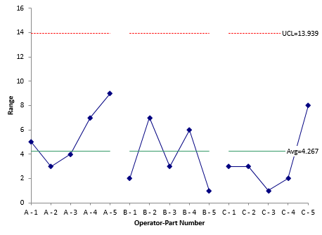
The X-R charts for the data are shown below. The range chart is shown in Figure 1.
Figure 1: Range Chart for Operator-Part Subgroups
With the range chart, you are looking to ensure that all ranges are consistent. Each range is a measure of the repeatability for an operator. If there are no points beyond the upper control limit (UCL), then you can say that the range chart is in statistical control – and conclude that the repeatability of each operator is the same. If there are any range values above the UCL, you need to find out why – what caused the point to be above the UCL.
The chart in Figure 1 is in statistical control – no points beyond the UCL. The repeatability variance can then be estimated from the average range shown on the chart:
where d2 is a control chart constant that depends on subgroup size. In this chart, the subgroup size is the number of trials (2). The value of d2 for a subgroup size of 2 is 1.128. For a list of control chart constants, please see our first X-R publication. The repeatability variance is then given by:

-
Operator A: 5.6
-
Operator B: 3.8
-
Operator C: 3.4
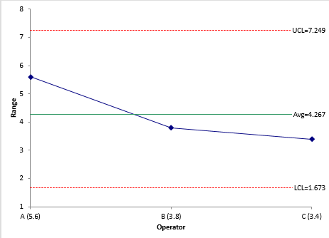
These three ranges are plotted on the mean range chart as shown in Figure 2. The overall average range from Figure 1 is plotted as the center line. Then the control limits are added. The control limits are given by:
UCL = UMR0.05(R)
LCL = LMR0.05(R)
where UMR0.05 and LMR0.05are scaling factors that depend on k, n and o. The 0.05 is the confidence coefficient. For k = 15, n = 2 and o = 3, the values are UMR0.05 = 1.699 and LMR0.05 = 0.392. A table of these values are available in Dr. Wheeler’s book reference above. Then:
UCL = UMR0.05(R)= 1.699(4.267) = 7.249
LCL = LMR0.05(R)= 0.392(4.267) = 1.673
These limits are added to Figure 2 as shown below. All three operator average ranges are within the control limits confirming that the operators have the same repeatability.
Figure 2: Mean Range Chart
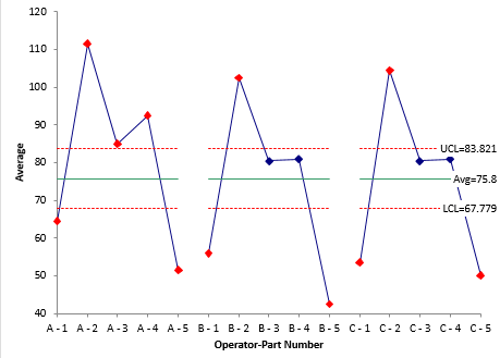
The X chart is shown in Figure 3. What does this X chart tell you? You are looking to see if operators appear to have the same results for each part.
Figure 3: X Chart for the Operator-Part Subgroups
Remember, the control limits for the X chart are based on the average range from the range chart in Figure 1. This average range is based on the repeatability of the operators. If the repeatability is small, then the control limits on the X chart should be tight and there should be out of control points.
It is the out of control points that you want to focus on. The points within the control limits are essentially “masked” by the measurement system repeatability. From Figure 3, it appears that operator A has higher average results than the other two operators.

-
Operator A: 81.0
-
Operator B: 72.5
-
Operator C: 73.9
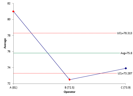
These three averages are plotted on the main effects chart as shown in Figure 4.
Figure 4: Main Effects Chart
The overall average from Figure 2 is plotted as the center line. Then the control limits are added. The control limits are given by:
UCL = Overall Average + ANOME0.05(R)
LCL = Overall Average + ANOME0.05(R)
where ANOME0.05 is a scaling factor that depends on k, n, and o. For k = 15, n = 2, and o = 3, the value of ANOME0.05 is 0.589. Thus,
UCL = Overall Average + ANOME0.05(R) = 75.8 + 0.589(4.267) = 78.313
LCL = Overall Average + ANOME0.05(R)= 75.8 – 0.589)4.267) = 73.287
These control limits are added as shown in Figure 4. Figure 4 shows that operator A and B have points beyond the control limits. Looking closer at the chart, it appears that operators B and C have similar results and operator A is the one that is different. This confirms what was seen in the X chart (Figure 3).
Out of control points in the mean range chart (Figure 2) or the main effects chart (Figure 4) will increase the % of the variation due to the measurement system (the % Gage R&R). Reasons for these out of control points should be investigated and corrected. The Gage R&R study would then need to be repeated.
Step 2: Calculate the Repeatability Variance
We already did this in step 1 using the average range from Figure 1. The repeatability variance is given by:
Step 3: Calculate the Reproducibility Variance
The three operator averages are used to estimate the reproducibility variance. The equation to calculate this variance is:
where R0 is the range of the operator averages and d2* is a bias correction factor that depends on the number of operators. The value of R0 for the three operators is 81 – 72.5 = 8.5. The value of d2* for three operators is 1.906.
Step 4: Calculate the Combined R&R Variance
The combined R&R variance is the sum of the repeatability variance and the reproducibility variance:
Step 5: Calculate the Product Variance
The range of the p part averages is used to determine the product variance using the following:
where Rp is the range of the part averages d2* is a bias correction factor that depends on the number of parts. The part averages are Part 1 = 58, Part 2 = 106.167, Part 3 = 82, Part 4 = 84.833, and Part 5 = 48. The value of Rp is 58.167. The value of d2* is 2.477 for five parts.
Step 6: Calculate the Total Variance
The total variance is the sum of the product variance and the combined Gage R&R variance:
Step 7: Calculate the Fraction of the Total Variance due to Repeatability
This is the ratio of the repeatability variance to the total variance.
Step 8: Calculate the Fraction of the Total Variance due to Reproducibility
This is the ratio of the reproducibility variance to the total variance.
Step 9: Calculate the Fraction of the Total Variance due to the Combined R&R
This is the ratio of the combined R&R variance to the total variance.
Step 10: Calculate the Fraction of the Total Variance due to the Product Variance
This is the ratio of the product variance to the total variance.
Note: this is the value the intraclass correlation coefficient (r).
Step 11: Interpret the Results
This is the key – all the calculations have been done. But what do they mean? Dr. Wheeler uses the table below to interpret the results.
Table 3: Interpreting the EMP Results
| Intraclass coefficient | Type of Monitor | Reduction of Process Signal | Chance of Detecting ± 3 Std. Error Shift | Ability to Track Process Improvements |
|---|---|---|---|---|
| 0.8 to 1.0 | First Class | Less than 10% | More than 99% with Rule 1 | Up to Cp80 |
| 0.5 to 0.8 | Second Class | From 10% to 30% | More than 88% with Rule 1 | Up to Cp50 |
| 0.2 to 0.5 | Third Class | From 30% to 55% | More than 91% with Rules 1, 2, 3 and 4 | Up to Cp20 |
| 0.0 to 0.2 | Fourth Class | More than 55% | Rapidly Vanishing | Unable to Track |
This table was described in detail in our first publication on EMP. Please refer to that publication for more information. The first column lists the value of the Intraclass Correlation Coefficient. The second column lists whether it is a First Class, Second Class, Third Class or Fourth Class monitor – with “First” being the best.
Since the value of r from the Gage R&R study in this publication is 0.994, the measurement system for thickness is a First Class Monitor. This means that there is less than a 10% reduction in a process signal, there is a better than 99% chance of detecting a point beyond the control limits (Rule 1) and that the measurement system will be able to track process improvements up to Cp80. Cp80 is calculated based on specifications and marks the point from the measurement system will move from a first class to a second class monitor. Again, the details of this table are in our previous publication. But everything points to the thickness measurement system being very good.
Table 4 below summarizes the variance calculations for this Gage R&R study.
Table 4: Components of Variance Results
| Component | Variance | % of Total |
|---|---|---|
| Repeatability | 14.307 | 2.5% |
| Reproducibility | 18.457 | 3.2% |
| R&R | 32.765 | 5.6% |
| Product | 549.053 | 94.4% |
| Total | 581.818 |
The % values given in this table are similar to what you would get from the ANOVA method for analyzing a Gage R&R. Most people just focus on the value of % of variance due to the Gage R&R (5.6% here). If this value is less than 10%, they assume the measurement system is acceptable. What is acceptable? The % R&R value by itself does not mean much. That is why using Table 3 above to interpret the results is so valuable.
Summary
This month’s publication looked at Dr. Wheeler’s “Honest Gage R&R Study” procedure. This methodology involves using control charts to ensure that the results are consistent and predictable and that there is not bias in the operator averages or differences in the operator repeatability. The various components of variance are then calculated.
The intraclass correlation coefficient, which is the ratio the product variance to the total variance, is used to determine if the measurement systems is a First, Second, Third or Fourth class monitor. This designation allows you to determine how the measurement system reduces process signals and the probability that the measurement system will find shifts in the process. It also quantifies how much process improvement the measurement system can track before it moves to the next lower class of monitor.


Hi Bill,Thank you so much for your sharing. This is very helpful. I'just wonder that in GRR analysis we compare GRR value with process specification to see if it is significant different, but in Bias we just compare measured value with reference value by hypothesis test, not with specification. In some cases, the bias is large (hypothesis fail) but the process specification is too high so can we still accept the bias of measurement system ?Regards, Duy
The bias test is designed to tell if you have bias present. You can chose not to worry about it if you want ti due to the specifications. So, you are looking at two different things with the two methodologies.
Thank for your quick reply and your information. For example, the bias of two measurement system is 0.15 (fail hypothesis test) but the product specification is 2. % contribution of bias/specification is <10% (7.5%) so I decide to not worry about it. I'm not sure about my justification method because it is not related to any standard but in manufacturing partical we use it alot. The hypothesis test is very easy to fail and we can not adjust the system day to day due to cost and lead time (especially the product tolerance is high like example above). Could you share me the better way to deal with situation ?
Dear Bill. My name is Junho Kim. I am working as a software engineer. I have question while using Gage R&R in MSA analysis of SPC for Excel. We are only interested in the %Tolerance value and NDC value However, we want to study with only one Operator The %Tolerance value and NDC value were not found in the EMP analysis Please tell me how to get %Tolerance value and NDC value in One Operator’s condition I’m looking forward your reply soon. Thank you.
A gage R&R analysis has more than one operator – only way to determine the impact of different operators. You can do it with one operator (Consistency Study) but that will not give you NDC or % tolerance. But you can use the equations to determine those two values.