January 2018
(Note: all the previous SPC Knowledge Base in the measurement systems analysis category are listed on the right-hand side. Select this link for information on the SPC for Excel software.)

This publication examines the impact of measurement error on its ability to detect a process shift. It demonstrates that a measurement system that is responsible for 50% of the total variance can still detect signals from a control chart that something in the process has changed. This, by itself, shows the fallacy of setting these somewhat arbitrary standards for what makes a measurement system acceptable.
Instead, we need a method of classifying a measurement system that makes sense in terms of our process. Dr. Donald Wheeler has developed such a system. This method of classifying a measurement system is covered in this publication.
In this issue:
- Relationship between Total, Product and Measurement Variation
- An “Acceptable” Measurement System
- Control Chart Tests
- The Perfect Measurement System
- Adding in Measurement Error
- Dr. Wheeler’s Method of Classifying a Measurement System
- Summary
- Quick Links
Please feel free to leave a comment at the end of the publication. You can download a pdf copy of this publication at this link.
Relationship between Total, Product and Measurement Variation
You take a sample from your process. You test that sample using your measurement system. You get a result (X1). You take another sample and test that sample. You get another result (X2). Usually X1 does not equal X2. What are in these results? Two major components are present in each result: the variation in the product itself and the variation in the measurement system.
The basic equation describing the relationship between the total variance, the product variance and the measurement system variance is given below.
σx2= σp2+σe2
whereσx2= total variance of the product measurements,σp2= the variance of the product, andσe2= the variance of the measurement system.
The % variance to the measurement system is simply the following ratio:
% variance due to the measurement system = 100(σe2/σx2)
An “Acceptable” Measurement System
There are several ways of determining the total, product and measurement system variances. Regardless of how the variances are calculated, what is an acceptable number for % variance due to the measurement system? AIAG recommends the following:
- Less than 1%: The measurement system is acceptable.
- Between 1% and 9%: The measurement system is acceptable depending on the application, the cost of the measurement device, cost of repair, or other factors.
- Greater than 9%: The measurement system is not acceptable and should be improved.
One of our earlier publications contains the following statement:
A precise measurement system is defined as one that is in statistical control with respect to variation (i.e., the range chart) and that is responsible for less than 10% of the total process variance.
I don’t agree with the 10% anymore. It seems like a good goal, but measurement systems can have significantly larger values and still be very useful. After all, a major reason for taking measurements is to see if something has changed. At the heart of this is the control chart. The control chart will send you a signal if the process has changed.
Why my change of heart on what makes a measurement system acceptable? His name is Dr. Donald Wheeler and the book is “EMP III: Evaluating the Measurement Process.” He has developed a great method for classifying how useful a measurement system is. This publication is based on some of the material in Chapter 15 of his book. If you don’t have this book, you should get it (www.spcpress.com).
Control Chart Tests
In the analysis below, we will be interpreting control charts. To find signals on the control charts, we will use these four Western Electric zone tests:
- Rule 1: a point is beyond the lower or upper control limit
- Rule 2: two out of three consecutive points on the same side of the average are more than two standard deviations away from the average
- Rule 3: four out of five consecutive points on the same side of the average are more than one standard deviation away from the average
- Rule 4: Eight consecutive points are above or below the average
The Perfect Measurement System
Now suppose there is a perfect measurement system. It always generates the same result for a sample. It has no variation. Then the % of variation due to the measurement system is 0. This is the best it can be – never attainable though.
Let’s investigate how this perfect measurement system detects signals on a control chart. To begin, we need a stable, in control process. The random number generator in Excel was used to generate 80 random numbers from a normal distribution with an average of 0 and a standard deviation of 1.
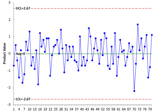
Figure 1 is the X control chart for the randomly generated values. These represent the product value since there is no measurement component. The control limits are based on the first 50 samples.
Figure 1: Product Values with No Measurement Error (Control Limits based on First 50 Samples)
This control chart is in statistical control. It is consistent and predictable. None of the four rules have been violated. The average is 0 which is right on the average used for the random number generation. The estimated sigma from the moving range chart (not shown here) is 0.88, close to the standard deviation (1) used for the random number generation.
Now we will add some signals to the control chart. We will look at 1, 2 and 3 sigma shifts in the average. Remember the control limits in Figure 1 are based on the first 50 samples. The following shifts will be added:
- Points 51 – 60: One sigma shift (add 1 to each point)
- Points 61 – 70: Two sigma shift (add 2 to each point)
- Points 71 – 80: Three sigma shift (add 3 to each point)
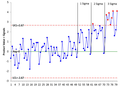
The resulting control chart with the shifts added is shown in Figure 2.
Figure 2: Product Values with Signals Added (No Measurement Error)
You can see the impact of the three shifts. The red points represent points beyond the control limits, which is Rule 1. The three shifts are divided by the vertical black lines.
Note that the 1 sigma shift does not have any points beyond the control limits. However, there are 8 points in a row above the average for that shift. So Rule 4 is violated and the control chart picks up the 1 sigma shift within 10 samples.
The 2 and 3 sigma shifts have points beyond the control limits. So with no measurement error, the shifts are easily picked up quickly.
Adding in Measurement Error
Measurement error has two impacts on the control chart. When it is present (as it always is), the control limits will be wider and it becomes more difficult to see the signals from the control charts. We are going to add in measurement error that is equal to the product variation above. This means the following is true:
% of total variance due to the measurement system = 50%
That is a lot of variation due to the measurement system. Surely this measurement system has too much variability. Well, according to the acceptance criteria above, it definitely does have too much variation since it is greater than 9%. But is it true that this measurement system has too much variability?
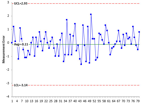
To add in measurement error, the random number generator in Excel was again used to generate 80 random numbers from a normal distribution with an average of 0 and a standard deviation of 1. The results are shown in Figure 3. Again, the control limits are based on the first 50 samples.
Figure 3: Measurement Error (Control Limits Based on First 50 Samples)
The average of the measurement error is – 0.11 which is close to the average (0) entered for the random number generation. The estimated standard deviation from the moving range chart (not shown here) is 1.01, which is close to the standard deviation (1) for the random number generation. The measurement error in Figure 3 is in statistical control.
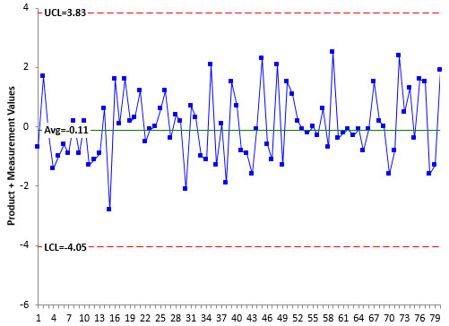
Now, the product values from Figure 1 and measurement error values from Figure 3 are added together to generate the results for a process with 50% measurement variation. These results are shown in Figure 4. The control limits have been recalculated and are based on the first 50 samples again.
Figure 4: Product Values + Measurement Error (Control Limits Based on First 50 Samples)
The combined control chart is in statistical control. The first thing to note is that adding measurement error increases the distance between the control limits. The more measurement error there is, the wider the control limits.
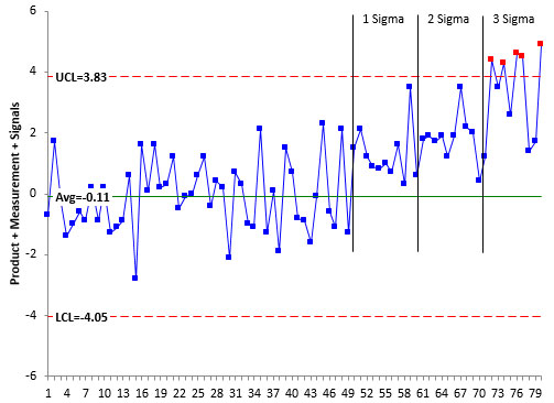
Now, the signals are added back in as above. Let’s see if a measurement system that is responsible for 50% of the total variance can pick up the shifts. The results are shown in Figure 5.
Figure 5: Product Values plus Measurement Error with Signals Added
All the points for the 1 and 2 sigma shifts are above the average this time. The measurement system, with its poor acceptability, still picks up the shifts using Rule 4. The 3 Sigma shift has points beyond the control limits.
So, should we be so quick to judge a measurement system as “bad” because it is responsible for 50% of the total variance. It still works – it sends us the signal that the process has changed.
In his book, Dr. Wheeler considered the perfect case, the case where the measurement system was responsible for 50% of the total variance and the case where the measurement system was responsible for 80% of the total variance. He considered shifts of 2, 3, 4, 5 and 6 sigma. He did not include the 1 sigma shift. In each of three cases, the control chart picked up the shifts – even the one where the measurement system was responsible for 80% of the total variance. Pretty amazing that the control chart can still deliver signals even with that much measurement error.
Dr. Wheeler’s Method of Classifying a Measurement System
It is obvious that the somewhat arbitrary method of saying a measurement system that is responsible for 10% or more of the total variance is unacceptable does not hold up in the light of the analysis above. What is really needed is a method of “judging” a measurement system based on how it actually performs in a control chart setting. Fortunately for us, Dr. Wheeler has supplied that method for us.
Dr. Wheeler’s method involves using the Intraclass Correlation Coefficient to determine the classification. The Intraclass Correlation Coefficient is simply the ratio of the product variance to the total variance and is denoted by :
ρ=σp2/σx2
This is simply the % of the total variance that is due to product variance. Remembering the basic equation above, then 1 –ρ is the % of the total variance that is due to the measurement system.
For more information on the variances are calculated, please see our two-part publication on Evaluating the Measurement System.
Dr. Wheeler uses the Intraclass Correlation Coefficient to place the measurement system into one of four classes. Table 1 summarizes these classes and the characteristics of those classes.
Table 1: The Four Classes of Process Monitors
| INTRACLASS COEFFICIENT | TYPE OF MONITOR | REDUCTION OF PROCESS SIGNAL | CHANCE OF DETECTING ± 3 STD. ERROR SHIFT | ABILITY TO TRACK PROCESS IMPROVEMENTS |
|---|---|---|---|---|
| 0.8 to 1.0 | First Class | Less than 10% | More than 99% with Rule 1 | Up to Cp80 |
| 0.5 to 0.8 | Second Class | From 10% to 30% | More than 88% with Rule 1 | Up to Cp50 |
| 0.2 to 0.5 | Third Class | From 30% to 55% | More than 91% with Rules 1, 2, 3 and 4 | Up to Cp20 |
| 0.0 to 0.2 | Fourth Class | More than 55% | Rapidly Vanishing | Unable to Track |
The first column lists the value of the Intraclass Correlation Coefficient. The second column lists whether it is a First Class, Second Class, Third Class or Fourth Class monitor – with “First” being the best. The example above with the measurement system being responsible for 50% of the total variance is on the border between a Second Class and Third Class monitor. Remember that the % of the variance due to the measurement system is 1 –ρ. So, as you move from a First Class to a Fourth Class monitor the % of variance due to the measurement system is increasing.
The third column shows how much of a reduction in a process signal there is. The First Class monitor has less than a 10% reduction in process signal while a Fourth Class monitor has more than a 55% reduction in process signal
The fourth column lists the chance of detecting a ± 3 standard error shift within ten samples. This is what we covered in this publication. Note that the First and Second Class monitors detect Rule 1 very well. Once you reach a Third Class monitor, you need to apply all four rules to keep the chance of detecting the shift high. Fourth Class monitors are not good at detecting any shifts essentially.
The fifth column describes the monitor’s ability to track process improvements. This is something we don’t think about too much. As we improve our processes, the variation due to the measurement system increases. This last column describes how much process improvement you can have until the measurement system moves from one class to another. Please see our two-part publication on Evaluating the Measurement System for more information on this.
Summary
This publication examined the impact of measurement error on a control chart’s ability to detect a process shift. It demonstrated that a measurement system that is responsible for 50% of the total variance can still detect signals from a control chart that something in the process has changed. This, by itself, demonstrated the fallacy of setting somewhat arbitrary standards for what makes a measurement system acceptable (like less than 9% of the total variance). Dr. Wheeler’s approach of classifying a measurement based on what the measurement system can really do is a much better approach.
Doesn't it seem odd that Dr. Wheeler defines a determination coefficient (r²) but names it as a correlation coefficient (r) ?Seriously, wouldn't "process determination coefficient" make a lot more sense than "Intraclass Correlation Coefficient" ?
Yes. I had not heard the term "Intraclass Correlation Coefficient" before reading his book. Might go along with his calling control imits "process behavior limits".
some though from a beginner who reads AIAG MSA manual recently, shouldn't it also considered the impac the measurement error has on process capability? if the measurement erro is way too large like the 50% example for instance, it would potentially make wrong decison (type 1 error?) agianst process capabiltiy or which is explained in appedix B of the MSA manual, that could be reaosn AIAG recommend the minimum measurement error should be 30% as the differnce between actual & obseved process capability is still acceptable. in other words, if the observed process capabiliy is 1.33 based on measurement error of 50%, the actual process capabilty could be higher than 1.33, so it will be no need to make any improvement on both measurement system of production process
The value of sigma used in the Cpk calculations of course contains measurement variation as well as process variation. If the measurement system variation is very high, you can work on reducing that to improve the process capability. But the actual process capability contains the variation due to the measurement system and the product – both. You can't separate them. Reducing variation in the product or the measurement system will both improve the process capability.