July 2016
(Note: all the previous SPC Knowledge Base in the basic statistics category are listed on the right-hand side. Select this link for information on the SPC for Excel software.)

You glance at the histogram of the data. Hmm. It looks a little skewed – a long tail towards the left. Maybe it is close enough to consider the data normal. You move to the normal probability plot. Oh no! The p-value is less than 0.05. It looks like your data may not be normal!
It makes some sense to you. The process has a lower bound of zero. The histogram shows skewed data. The points on the normal probability plot do not lie along the straight line. Yes, you have non-normal data.
But your customer wants that Cpk value – and that calculation requires the data to be normally distributed. Now what do you do? The month’s publication introduces a technique called the Box-Cox transformation. This technique attempts to transform your data in a way that the transformed values are normally distributed. If it is successful, you can then calculate your Cpk value.
In this issue:
- Introduction
- Modified Box-Cox Transformation
- Example Background Information
- Box-Cox Transformation Calculations
- Box-Cox Chart
- Checking the Box-Cox Transformation
- Process Capability Impact
- Minimize the Standard Deviation
- Summary
- Quick Links
Please feel free to leave a comment at the end of this publication. You may also download a pdf copy of this publication at this link.
Introduction
Some statistical tests are based on the assumption that your data are normally distributed. The process capability calculation involving Cpk is one of these. Sometimes, if your raw data are not normally distributed, you can transform the data to “make” the transformed values normally distributed. Then you can apply those tests that require a normal distribution.
When you transform a data set, you perform the same mathematical operation on each data point in the set. The Box-Cox transformation is power transformation that is defined by Yλ, where Y represents the data and λ is the “power” to which each data value is raised. It was introduced in 1964 by George Box and David Cox. The original form of the transformation was:
Y(λ) = (Yλ– 1)/λ when λ ≠ 0
Y(λ) = log(Y) when λ = 0
Sometimes (not always), this transformation will generate values that are normally distributed. The transformation examines values of λ between -5 and 5 to determine which value of λ fits the data best – in terms of making the transformed values normally distributed. Some common values of the λ are shown in Table 1 along with the transformation.
Table 1: Values of λ and the Box-Cox Transformation
| λ | Transformation |
| -2 | Y’= 1/Y2 |
| -1 | Y’ = 1/Y |
| -0.5 | Y’ = 1/SQRT(Y) |
| 0 | Y’ = LOG(Y) |
| 0.5 | Y’ = SQRT(Y) |
| 1 | Y’ = Y |
| 2 | Y’ = Y2 |
For example, if λ = 2, then the data are transformed by multiplying each data point by itself (Y2).
Modified Box-Cox Transformation
The original Box-Cox transformation has been modified over the years. Suppose you have a data set consisting of n values of Y. For this publication, we will use the transformation that includes the geometric mean as shown below.
Y(λ) = (Yλ– 1)/(λGMλ-1) when λ ≠ 0
Y(λ) = GM(ln(Y)) when λ = 0
GM=(Y1Y2Y3…..Yn)1/n
where GM is the geometric mean of the n Y values. The geometric mean is used as a scaling factor in this modified transformation. The example below shows how the Box-Cox transformation is done.
Example Background Information
During a test production run, 100 samples were taken. The data are shown in Table 2. To get production run order from the table, go down by columns. Sample 1 is 0.76, followed by sample 2 which is 6.26.
There is no lower specification limit (LSL) in this process, but there is a natural boundary of 0. So, the data cannot be less than or equal to 0. The upper specification limit (USL) for our process is 7.5.
Table 2: Production Data
| 0.76 | 2.85 | 2.64 | 2.44 | 4.64 | 5.31 | 5.79 | 3.80 | 6.08 | 0.44 |
| 6.26 | 1.12 | 2.57 | 2.87 | 6.97 | 3.24 | 1.60 | 4.23 | 2.56 | 3.07 |
| 1.01 | 2.06 | 0.43 | 1.05 | 2.19 | 2.21 | 1.41 | 2.85 | 1.75 | 7.03 |
| 0.71 | 1.67 | 3.08 | 3.38 | 2.49 | 1.92 | 0.64 | 0.78 | 2.40 | 4.69 |
| 5.05 | 4.96 | 4.24 | 3.44 | 2.24 | 7.09 | 2.90 | 0.57 | 4.15 | 2.78 |
| 0.28 | 1.63 | 4.14 | 3.51 | 4.79 | 3.95 | 4.33 | 4.99 | 3.01 | 1.20 |
| 3.91 | 2.31 | 3.25 | 1.30 | 3.24 | 3.80 | 3.21 | 0.84 | 0.97 | 3.47 |
| 1.36 | 1.97 | 0.53 | 1.97 | 5.64 | 0.34 | 2.12 | 4.39 | 1.35 | 2.28 |
| 2.53 | 4.72 | 2.51 | 6.67 | 5.30 | 3.33 | 2.58 | 1.13 | 1.14 | 2.45 |
| 3.83 | 0.84 | 4.23 | 4.28 | 0.76 | 6.33 | 3.48 | 1.35 | 1.23 | 1.22 |
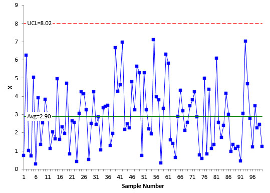
The first step in examining data is almost always to plot the data over time to see if the process is stable – consistent and predictable. If not, then your results have no meaning. The samples were analyzed using an individuals control chart to ensure that the process was stable. The X chart is shown in Figure 1.
Figure 1: X Control Chart
Each individual value is plotted on the X control chart. The average is then calculated along with the control limits. In this example, it is not possible to have values 0 or below. So, there is not a lower control limit. As long as all the samples are below the upper control limit and there are no patterns, the process is said to be stable – it is consistent and predictable – in statistical control.
This is the case in Figure 1. For more information on individual control charts, please see our publication at this link.
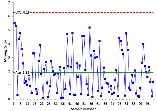
Figure 2 is the moving range control chart for the data. The moving range control chart plots the range between consecutive values. For example, the first point plotted is the range between the first two values in Table 1. The range is |0.76 – 6.26| = 5.5.
Figure 2: Moving Range Control Chart
The average moving range is calculated and added to the control chart along with the upper control limit. As long as there are no points beyond the upper control limit, the moving range control chart is in statistical control – it is consistent and predictable. This is the case for Figure 2.
Since the moving range chart is in control, the process standard deviation (σ) can be estimated using the following equation:
σ=R/1.128 =1.92/1.128=1.70
This is the measure of variation in the individual results. It is important to understand how this is calculated because, in this example, this is the measure of variation you want to minimize when running the Box-Cox transformation. This is how the Box-Cox transformation determines the best value of λ.
From the individuals control chart, you know that the process is consist and predictable. But are the data normal? This process for determining if your data are normal was covered in last month’s publication at this link. It involves using a histogram and a normal probability plot. Remember, the control chart was used to help ensure that the process was stable when the data were taken.
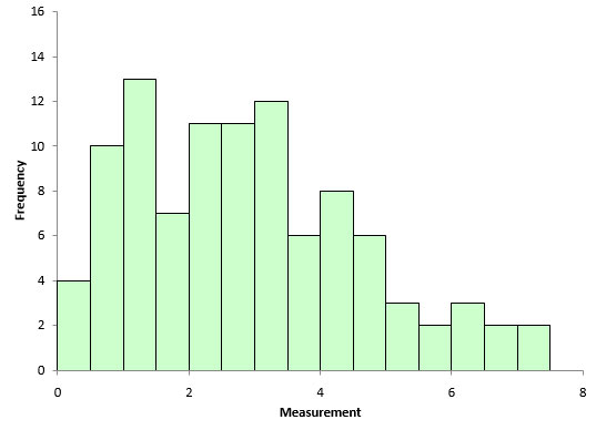
Figure 3 is a histogram of the 100 data points in Table 1. Does it “look” normal to you? Remember, for a normal distribution, you expect the distribution to be symmetrical. Does this histogram look symmetrical?
Figure 3: Histogram of Data
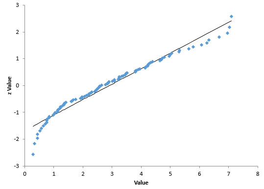
The histogram looks a little skewed. This is not surprising since we know the process has a lower bound of 0. And the process seems to operate closer to 0 most of the time. A normal probability plot was made as a final check. It is shown in Figure 4.
Figure 4: Normal Probability Plot
If the data came from a normal distribution, it would lie along the straight line shown in Figure 4. It does not do this. Plus, the p-value associated with this normal probability plot is 0.0131. Since this is below 0.05, we conclude that the data does not come from a normal distribution.
To calculate that Cpk value our customer wants for process capability, we need to try to transform the data to a normal distribution. This is where the Box-Cox transformation comes in.
Box-Cox Transformation Calculations
The Box-Cox calculation procedure is described below. Essentially, you are searching for the value of λ between -5 and 5 that minimizes the variation (σ). For each value of λ, you do the following:
- Transform the data using the modified Box-Cox transformation
- Calculate the moving range
- Estimate the value of σ as shown above
The value of λ that gives the smallest σ is the optimum λ value. The calculations are explained below for λ = 2. To start the transformation, you need the geometric mean of all the data. The geometric mean of the data in Table 1 is 2.3215. You can use the built-in Excel function GEOMEAN to calculate this.
The first data point is 0.76 in Table 1. The calculation to transform this data point is shown below:
Y(λ) = (Yλ– 1)/(λGMλ-1) = (Y2– 1)/(2(2.3215)2-1) = -0.090976
This calculation is repeated for each data point. The moving ranges are then calculated and the process standard deviation estimated using:
σ=R/1.128
This process is repeated for each value of λ. So each value of λ has a σ value associated with it.
Box-Cox Chart
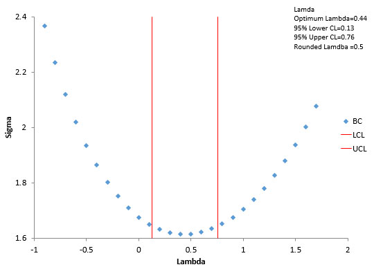
The Box-Cox chart is a plot of the λ values against the σ values. The plot for the data in this example is shown in Figure 5 (for a partial range between -5 and 5).
Figure 5: Box-Cox Chart
This plot helps identify where the minimum value of sigma lies. In the calculations, the actual minimum occurred at λ = 0.44. This is called the optimum lambda. All things vary. So do these results. The Box-Cox plot contains two other lines: the upper confidence limit and the lower confidence limit. The range between the confidence limits contain the potential values of λ that minimize the variation. We will not cover the calculation of the confidence limits here.
If the confidence interval contains an integer (e.g., 2, -2) or 0.5 or -0.5, then the value of λ is usually set to that value. The confidence interval in Figure 5 is from 0.13 to 0.76. This range contains 0.5. So, the transformation is taken to be:
Y(λ) = Y0.5
Each data point is transformed using the above equation. So, for the first data point:
Y(λ) = 0.760.5= 0.87178
Now, here is the thing to remember: just because you found a minimum sigma does not mean it transforms the data into a normal distribution. You have to check that.
Checking the Box-Cox Transformation
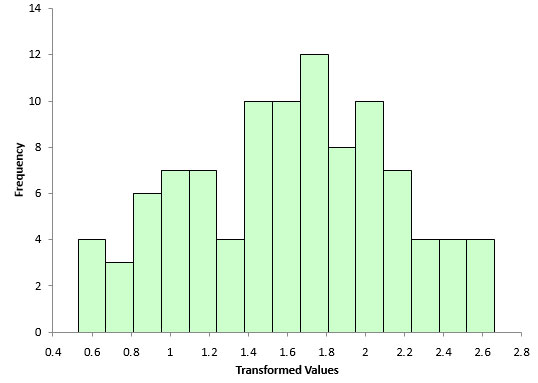
To check that the transformation produces a normal distribution, you can simply make a histogram and a normal probability plot using the transformed data. Figure 6 is the histogram of the transformed data.
Figure 6: Histogram of Transformed Data
Compare this histogram to the one in Figure 3. You can see that this histogram looks more bell-shaped. It appears that the transformation may have worked. You can confirm this by doing a normal probability plot as shown in Figure 7.
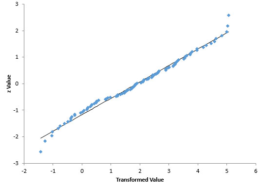
Figure 7: Normal Probability Plot of Transformed Data
Compare this normal probability plot to the one in Figure 4. It appears that this one fits the straight line better. The p-value for this plot is 0.45. Since it is greater than 0.05, you conclude that the data come from a normal distribution. The Box-Cox transformation with λ = 0.5 does transform the original data to a normal distribution.
Process Capability Impact
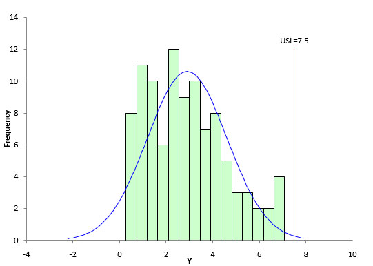
The upper specification for our process is 7.5. Figure 8 shows the process capability analysis performed on the raw data (no transformation). You can see that the histogram does not look normal. But the Cpk calculations requires the normal distribution. You can see that the tail on the distribution extends below 0 – but our process has a natural boundary that prevents that. The Cpk value for Figure 8 is 0.9.
Figure 8: Process Capability Based on Raw Data
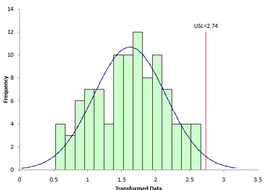
The key for Figure 8 is that the calculation for Cpk is not valid since the data are not normally distributed. Figure 9 is the process capability chart based on the transformed data. The histogram looks much more normal and the data does not extend below 0. The Cpk for this process analysis is 0.7.
Figure 9: Process Capability Based on Transformed Data
With Figure 9, the Cpk calculation is valid. The transformed data are normally distributed.
Minimize the Standard Deviation
The procedure for the Box-Cox transformation is to find the value of λ between -5 and 5 that minimizes the standard deviation of the transformed data. But, there are multiple ways to estimate a standard deviation. What is the best way? It depends on the data you have – and it is not just the calculated standard deviation of all the data.
If you have individual values, then the average moving range is used to estimate the standard deviation. This is what we did in the example above.
However, if you are subgrouping your data to monitor the process, then you will want to minimize the estimated standard deviation based on the subgroup range or subgroup standard deviation control chart. You could also use the pooled variance.
Summary
This month’s publication introduced the Box-Cox transformation. This transformation attempts to transform a set of data to a normal distribution by finding the value of λ that minimizes the variation. This allows you to perform those calculations/tests that require the data to be normally distributed – like the calculation of Cpk. The Box-Cox transformation does not always convert the data to a normal distribution. You must check the transformation to ensure it worked.
