Control Limits – Where Do They Come From?

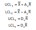
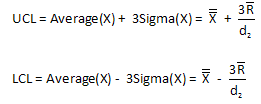
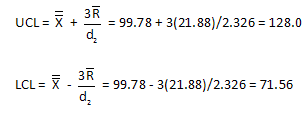
Ever wonder where the control limit equations come from? We use two statistics, the overall average and the average range, to help us calculate the control limits. For example, the control limit equations for the classical Xbar-R control chart are:

What is A₂ and where does it come from? How is it related to the overall average and the average range? What about D₄ and D₃? This newsletter is designed to answer these questions. The information in this newsletter is adapted from Dr. Don Wheeler’s book Advanced Topics in Statistical Process Control (www.spcpress.com).

In this issue:

• Control Limit Equations
• Distributions
• The Data
• Distribution of Individual Values
• Distribution of Subgroup Averages
• Distribution of Subgroup Ranges
• d₂ and d₃
• Generating the Control Limits
• Quick Links

Control Limit Equations

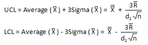
Control limit equations are based on three sigma limits. Just remember, it is three sigma limits of what is being plotted. So, what does that mean? If you are plotting individual values (e.g., the X control chart for the individuals control chart), the control limits are given by:

UCL = Average(X) + 3*Sigma(X)

LCL = Average(X) – 3*Sigma(X)

where Average (X) = average of all the individual values and Sigma(X) = the standard deviation of the individual values.

If you are plotting subgroup averages (e.g., the Xbar control chart), the control limits are given by:

UCL = Average(Xbar) + 3*Sigma(Xbar)

LCL = Average(Xbar) – 3*Sigma(Xbar)

where Average(Xbar) = average of the subgroup averages and Sigma(Xbar) = the standard deviation of the subgroup averages.

If you are plotting range values, the control limits are given by:

UCL = Average(R)+ 3*Sigma(R)

LCL = Average(R) – 3*Sigma(R)

where Average(R)= average of the range values and Sigma(R) = standard deviation of the range values.

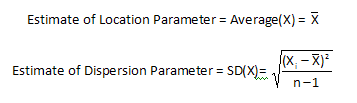
So for each set of control limits, there is a location parameter and a dispersion parameter. The location parameter simply tells us the average of the distribution. The dispersion parameter gives us the amount of variation in the data. The average is an estimate of the location parameter. The standard deviation is an estimate of the dispersion or variation parameter.

Distributions

There are three distributions to consider when discussing the control limit equations. These are:

• Distribution of the individual values
• Distribution of the subgroup averages
• Distribution of the subgroup ranges

Each of these three distributions has a location parameter (the average) and a dispersion parameter (standard deviation). We will take a look at what these parameters are and how they are used in the control limit equations. We will use data to develop estimates of both these parameters.

The Data

To start, 100 subgroups of size 5 were generated in Microsoft Excel using the random number generator (must install the Analysis Tookpak add-in). The average used in the random number generator was 100 with a standard deviation of 10. You can download the workbook containing the data here: download workbook . Since this a random number generator, it should generate a sequence of normally distributed numbers that is stable (i.e., in statistical control).

The first five subgroups from the data are shown below.

Subgroup Number	Sample 1	Sample 2	Sample 3	Sample 4	Sample 5	Subgroup Average	Subgroup Range
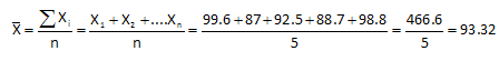
1	99.6	87.0	92.5	88.7	98.8	93.32	12.6
2	89.7	92.9	96.3	101.7	104.9	97.10	15.2
3	91.3	89.9	90.0	118.5	85.2	94.98	33.3
4	106.3	104.5	120.8	97.1	102.8	106.3	23.7
5	111.6	74.3	87.9	118.9	97.0	97.94	44.6

For each subgroup, the subgroup average was calculated. For example, for subgroup 1, the subgroup average is given by:

The subgroup range for the first subgroup is given by:

R = Maximum – Minimum = 99.6 – 77 = 12.6

This was done was all 100 subgroups. We can construct histograms to explore the three distributions referenced above.

Distribution of Individual Values

The histogram for the distribution of individual values is shown below in Figure 1.

 

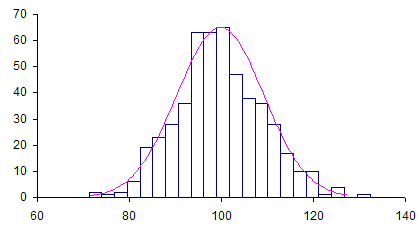
A normal curve has been superimposed on the histogram. As expected, the individual values are normally distribution. The location parameter for this distribution (histogram) is simply the average of the data. The dispersion parameter is the standard deviation of the data. The calculated average of the data is 99.78; the standard deviation (from using STDEV function in Excel) is 9.50. Both these values are close to the average and standard deviation used in the random number generator. For the individual values, where n is the subgroup size:

Distribution of Subgroup Averages

The histogram for the distribution of subgroup averages is shown below in Figure 2.

Figure 2: Distribution of Subgroup Averages

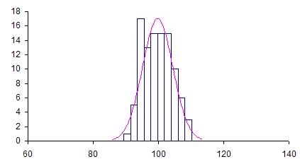
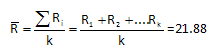
This distribution is also normally distributed as one would expect. The same x-axis scale was used for both Figure 1 and Figure 2. Note that the subgroup averages have less variation that the individual values. The location parameter for this distribution is the overall average defined as the following:

 

The dispersion parameter is given by the standard deviation of the Xbar values, where k is the number of subgroups.

 

 

 

The values above were obtained using the data for the 1000 subgroups. Again, you can download that workbook here. So, for the subgroup averages:

A couple of items to note at this point:

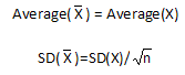
The standard deviation of the subgroup average is equal to the standard deviation of the individual values divided by the square root of the subgroup size. Note that if you perform the calculation with the above data you will get 4.25 for the standard deviation of the subgroup averages. It is not exact but close to 4.39. This is due to using data to estimate the parameters.

Distribution of Range Values

The distribution of range values is shown in Figure 3.

Figure 3: Distribution of Range Value

 

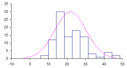
A normal distribution has been superimposed over the ranges. But note that the range values are not normally distributed. They are skewed. This is true of measures of dispersion (variation). For example, if you construct a histogram using the subgroup standard deviations, the distribution will also be skewed. The location parameter for the range distribution is simply the average range:

But what about an estimate of the dispersion parameter for the range values, SD(R)? This is where we have to turn to some theoretical values: d₂ and d₃.

d₂ and d₃

There is a paper (Tables of Range and Studentized Range, written by H. Leon Harter from 1960 that gives the moments of the range for samples of subgroup n from a normal distribution. For those of you who are interested in the details and the complicated equations, you can download the paper here. The paper also gives some of the history of using subgroup ranges as measures of dispersions. The paper describes the numerical integration required to obtain two values: d₂ which is the expected value of the range and d₃ which is the standard deviation of that expected value. The two equations are:

d₂ = Average(R)/SD(X)

d₃ = SD(R)/SD(X)

The first equation, d₂, examines the ratio of the average range divided by the standard deviation of the individual X values. The next equation, d₃, examines the ratio of the standard deviation of the range values divided by the standard deviation of the X values. Both of these values are theoretical, based on taking samples of subgroup size n from a normal distribution. The values of d₂ and d₃ for subgroup sizes 2 to 10 are given below.

Values of d₂ and d₃

n	d2	d3
2	1.128	.8525
3	1.693	.8884
4	2.059	.8798
5	2.326	.8641
6	2.534	.8489
7	2.704	.8332
8	2.847	.8198
9	2.970	.8078
10	3.078	.7971

 

Generating the Control Limit Equations

Now with the theoretical values of d₂ and d₃, we can move forward with finding the control limit equations.

So,

Rearranging d₂ = Average(R)/SD(X) gives:

Using this estimate of Sigma(X) and  the fact that the standard deviation of the subgroup averages is equal to the standard deviation of the individual values divided by the square root of the subgroup size gives:

Rearranging d₃ = SD(R)/SD(X) and using the estimate of Sigma(X) gives:

 

Now that we have estimated the location and dispersion parameters, we can use them to construct the three sigma limits for the three histograms.

For the individual values, the control limits are:

 

For the individuals values given in the workbook and using d₂ = 2.326 for a subgroup size of 5 the control limits are:

 

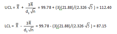
For the subgroup averages, the control limits are:

 

For the subgroup averages given in the workbook, the control limits are:

 

The control limits for the Xbar chart are usually written as shown at the start of this newsletter.  The equations contain the control chart constant A₂.  You can see from the equations above,  the following is true:

 

For the range chart, the control limits are:

 

 

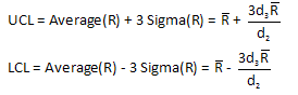
For the ranges given in the workbook, the control limits are:

 

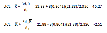
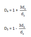
The control limits for the R chart are usually given as shown at the start of this newsletter.  Those limits include the control chart constants D₄ and D₃.  Using the equations above for the range control limits, it can be seen that the following are true:

So, you can see that the control limit equations depend on estimating two parameters from the process: the average as an estimate of the location parameter and the range as an estimate of the dispersion parameter. Then all you need for the control limits are the two theoretical values d₂ and d₃. These values depend on the subgroup size.