August 2012
 This month’s newsletter is the first in a multi-part series on using the ANOVA method for an ANOVA Gage R&R study. This method simply uses analysis of variance to analyze the results of a gage R&R study instead of the classical average and range method. The two methods do not generate the same results, but they will (in most cases) be similar.
This newsletter focuses on part of the ANOVA table and how it is developed for the Gage R &R study. In particular it focuses on the sum of squares and degrees of freedom. Many people do not understand how the calculations work and the information that is contained in the sum of squares and the degrees of freedom. In the next few issues, we will put together the rest of the ANOVA table and complete the Gage R&R calculations.
In this issue:
- Sources of Variation
- Example Data
- The ANOVA Table for Gage R&R
- The ANOVA Results
- Total Sum of Squares and Degrees of Freedom
- Operator Sum of Squares and Degrees of Freedom
- Parts Sum of Squares and Degrees of Freedom
- Equipment (Within) Sum of Squares and Degrees of Freedom
- Interaction Sum of Squares and Degrees of Freedom
- Summary
- Quick Links
Any gage R&R study is a study of variation. This means you have to have variation in the results. On occasion, I get a phone call from a customer wondering why their Gage R&R study is not giving them any useful information. And, in looking at the results, I discover that each result is the same – for each part and for each operator. There is no variation. I am asked – Isn’t it good that there is no variation in the results? No, not in a gage R&R study. It means that the measurement process cannot tell the difference between the samples. So remember, a gage R&R study is a study in variation – this means that there must be variation.
If you are not familiar with how to conduct a Gage R&R study, please see our December 2007 newsletter. This newsletter also includes how to analyze the results using the average and range method.
As usual, please feel free to leave comments at the end of the newsletter.
Sources of Variation
 Suppose you are monitoring a process by pulling samples of the product at some regular interval and measuring one critical quality characteristic (X). Obviously, you will not always get the same result when measure for X. Why not? There are many sources of variation in the process. However, these sources can be grouped into three categories:
- variation due to the process itself
- variation due to sampling
- variation due to the measurement system
These three components of variation are related by the following:
![]()
where σt2is the total process variance; σp2is the process variance; σs2is the sampling variance and σms2is the measurement system variance. Note that the relationship is linear in terms of the variance (which is the square of the standard deviation), not the standard deviation.
For our purposes here, we will ignore the variance due to sampling (or more correctly, just include it as part of the process itself). However, for some processes, sampling variation can greatly impact the results. Thus, we will consider the total variance to be:
![]()
Remember geometry? The right triangle? The Pythagorean Theorem? The above equation can be represented by the triangle below.
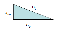
The total standard deviation, σt, for a measurement is equal to the length of the hypotenuse. The process standard deviation, σp, is equal to the length of one side of the triangle and the measurement system standard deviation, σms, is equal to the length of the remaining side.
You can easily see from this triangle what happens as the variation in the product and measurement system changes. If the product standard deviation is larger than the measurement standard deviation, it will have the larger impact on the total standard deviation. However, if the measurement standard deviation becomes too large, it will begin to have the largest impact.
Thus, the objective of improving a measurement system is to minimize the % variance due to the measurement system:
% Variance due to measurement system = 100(σms2/σt2)
The gage R&R study focuses on σms2. In a gage R&R study, you can break down σms2into its two components:
![]()
Repeatability is the ability of the measurement system to repeat the same measurements on the same sample under the same conditions. It represents an assessment of the ability to get the same measurement result each time.
Reproducibility is the ability of measurement system to return consistent measurements while varying the measurement conditions (different operators, different parts, etc.) It represents an assessment of the ability to reproduce the measurement of other operators.
In this series, we will take a look at how the repeatability and reproducibility are determined using the ANOVA method for Gage R&R.
Example Data
We will re-use the data from our December 2007 newsletter on the average and range method for Gage R&R. In this example, there were three operators who tested five parts three times. A picture of part of the Gage R&R design is shown below.
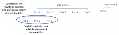
Operator 1 will test 5 parts three times each. In the figure above, you can see that Operator 1 has tested Part 1 three times. What are the sources of variation in these three trials? It is the measurement equipment itself. The operator is the same and the part is the same. The variation in these three trials is a measure of the repeatability. It is also called the equipment variation in Gage R&R studies or the “within” variation in ANOVA studies.
Operator 1 also runs Parts 2 through 5 three times each. The variation in those results includes the variation due to the parts as well as the equipment variation. Operator 2 and 3 also test the same 5 parts three times each. The variation in all results includes the equipment variation, the part variation, the operator variation and the interaction between operators and parts. The variation in all results is the reproducibility.
The data from the December 2007 newsletter are shown in the table below.
| Operator | Part | Results | ||
| A | 1 | 3.29 | 3.41 | 3.64 |
| 2 | 2.44 | 2.32 | 2.42 | |
| 3 | 4.34 | 4.17 | 4.27 | |
| 4 | 3.47 | 3.5 | 3.64 | |
| 5 | 2.2 | 2.08 | 2.16 | |
| B | 1 | 3.08 | 3.25 | 3.07 |
| 2 | 2.53 | 1.78 | 2.32 | |
| 3 | 4.19 | 3.94 | 4.34 | |
| 4 | 3.01 | 4.03 | 3.2 | |
| 5 | 2.44 | 1.8 | 1.72 | |
| C | 1 | 3.04 | 2.89 | 2.85 |
| 2 | 1.62 | 1.87 | 2.04 | |
| 3 | 3.88 | 4.09 | 3.67 | |
| 4 | 3.14 | 3.2 | 3.11 | |
| 5 | 1.54 | 1.93 | 1.55 | |
The operator is listed in first column and the part numbers in the second column. The next three columns contain the results of the three trials for that operator and part number. For example, the three trial results for Operator A and Part 1 are 3.29, 3.41 and 3.64.
We will now take a look at the ANOVA table, which is used as a starting point for analyzing the results.
The ANOVA Table for Gage R&R
In most cases, you will use computer software to do the calculations. Since this is a relatively simple Gage R&R, we will show how the calculations are done. This helps understand the process better. The software usually displays the results in an ANOVA table. The basic ANOVA table is shown in the table below for the following:
- k = number of operators
- r = number of replications
- n= number of parts
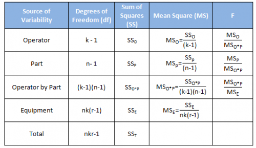
The first column is the source of variability. Remember that a Gage R&R study is a study of variation. There are five sources of variability in this ANOVA approach: the operator, the part, the interaction between the operator and part, the equipment and the total.
The second column is the degrees of freedom associated with the source of variation. The degrees of freedom are simply the number of values of a statistic that are free to vary. For example, suppose you have a sample that contains n observations. We use the sample to estimate something – usually an average. When we want to estimate something, it costs us one degree of freedom. So, if we have n observations and want to estimate the average, then we have n – 1 degrees of freedom left.
The third column is the sum of squares (SS) associated with the source of variation. The sum of squares is a measure of variation. It measures the squared deviations around an average. Remember what the equation for the variance is? The variance of a set of number is given by:
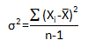
The sum of squares for the source of variation is very similar to the numerator. You just take the sum of squares around different averages depending on the source of variation.
The fourth column is the mean square associated with the source of variation. The mean square is the estimate of the variance for that source of variability based on the amount of data we have (the degrees of freedom). So, the mean square is the sum of squares divided by the degrees of freedom. Note the similarity to the formula for the variance above.
The fifth column is the F value. This is the statistic that is calculated to determine if the source of variability is statistically significant. It is the ratio of two variances (or mean squares in this case).
The ANOVA Results
The data above were analyzed using the SPC for Excel software. The resulting ANOVA table is shown below.
| Source | df | SS | MS | F | p Value |
| Operator | 2 | 1.630 | 0.815 | 100.322 | 0.0000 |
| Part | 4 | 28.909 | 7.227 | 889.458 | 0.0000 |
| Operator by Part | 8 | 0.065 | 0.008 | 0.142 | 0.9964 |
| Equipment | 30 | 1.712 | 0.057 | ||
| Total | 44 | 32.317 |
Let’s see where the numbers come from.
Total Sum of Squares and Degrees of Freedom
The total sum of squares (SST) is the sum of the other sources of variability. So,
SST = SS0 + SSP + SS0*P + SSE
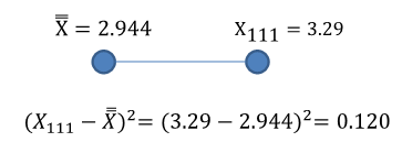
The total sum of squares is the squared deviation of each individual result from the overall average – the average of all results. The overall average of the 45 results is:
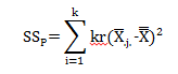
The total sum of squares is then given by:
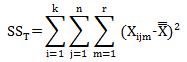
where Xijm is the result for the ith operator running the jth part for the mth trial. This equation is simply a fancy way of saying that you subtract the average from an individual result and square that result. This is shown in the figure below for the squared deviation of the first result.
If you do this for each point and add up the results, you will obtain the following:
SST = 32.317
The calculations are shown in the table below.
| Operator | Part 1 | Trial 1 | Trial 2 | Trial 3 | Squared Deviation Trial 1 | Squared Deviation Trial 2 | Squared Deviation Trial 3 |
| A | 1 | 3.29 | 3.41 | 3.64 | 0.120 | 0.217 | 0.485 |
| 2 | 2.44 | 2.32 | 2.42 | 0.254 | 0.389 | 0.274 | |
| 3 | 4.34 | 4.17 | 4.27 | 1.949 | 1.504 | 1.759 | |
| 4 | 3.47 | 3.5 | 3.64 | 0.277 | 0.309 | 0.485 | |
| 5 | 2.2 | 2.08 | 2.16 | 0.553 | 0.746 | 0.614 | |
| B | 1 | 3.08 | 3.25 | 3.07 | 0.019 | 0.094 | 0.016 |
| 2 | 2.53 | 1.78 | 2.32 | 0.171 | 1.354 | 0.389 | |
| 3 | 4.19 | 3.94 | 4.34 | 1.553 | 0.992 | 1.949 | |
| 4 | 3.01 | 4.03 | 3.2 | 0.004 | 1.180 | 0.066 | |
| 5 | 2.44 | 1.8 | 1.72 | 0.254 | 1.308 | 1.498 | |
| C | 1 | 3.04 | 2.89 | 2.85 | 0.009 | 0.003 | 0.009 |
| 2 | 1.62 | 1.87 | 2.04 | 1.752 | 1.153 | 0.817 | |
| 3 | 3.88 | 4.09 | 3.67 | 0.877 | 1.314 | 0.527 | |
| 4 | 3.14 | 3.2 | 3.11 | 0.039 | 0.066 | 0.028 | |
| 5 | 1.54 | 1.93 | 1.55 | 1.971 | 1.028 | 1.943 | |
| Sum | 32.317 | ||||||
There were a total of 45 results. We calculated the overall average for these results. So the degrees of freedom associated with the total sum of squares are 45 – 1 = 44. This can also be calculated as nkr – 1.
Operator Sum of Squares and Degrees of Freedom
As mentioned before, you obtain the sum of squares by determining the squared deviations between two numbers. With the operator source of variability, you will obtain the squared deviations between the operator average and the overall average. Algebraically, this is given by:

where nr represents the number of results for operator i and the “i..” subscript means over all parts and trials for operator i.
In this example, n = 5 and r = 3, so there are 15 results for each operator. The table below shows how the calculations are done:
| Operator | Parts | Trial 1 | Trial 2 | Trial 3 | Operator Average | Squared Deviation for Operator |
| A | 1 | 3.29 | 3.41 | 3.64 | 3.1567 | 0.0453 |
| 2 | 2.44 | 2.32 | 2.42 | |||
| 3 | 4.34 | 4.17 | 4.27 | |||
| 4 | 3.47 | 3.5 | 3.64 | |||
| 5 | 2.2 | 2.08 | 2.16 | |||
| B | 1 | 3.08 | 3.25 | 3.07 | 2.9800 | 0.0013 |
| 2 | 2.53 | 1.78 | 2.32 | |||
| 3 | 4.19 | 3.94 | 4.34 | |||
| 4 | 3.01 | 4.03 | 3.2 | |||
| 5 | 2.44 | 1.8 | 1.72 | |||
| C | 1 | 3.04 | 2.89 | 2.85 | 2.6947 | 0.0621 |
| 2 | 1.62 | 1.87 | 2.04 | |||
| 3 | 3.88 | 4.09 | 3.67 | |||
| 4 | 3.14 | 3.2 | 3.11 | |||
| 5 | 1.54 | 1.93 | 1.55 | |||
| Sum of Deviations | 0.1087 | |||||
| 15(Sum of Deviations) | 1.6304 | |||||
Thus,
SSO = 1.6304
So, you can see that the sum of squares due to the operators is based on how the operator averages deviate from the overall average. There are three operator averages. Since we calculated the overall average, we lost one degree of freedom. The degrees of freedom associated with the operators are 3 – 1 = 2, or k -1 = 2.
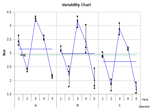
The variability chart below shows the results by operator by part. The horizontal blue line is the average for the operator. The horizontal green line is the overall average. The difference between those two lines is the deviation.
Parts Sum of Squares and Degrees of Freedom
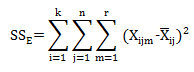
The sum of square due to the parts is done in the same manner as for the operators except the average you are focusing on are the part averages. Algebraically, the equation for SSP is:
where kr is the number of results for a given part (3 operators, 3 trials) and the subscript “.j.” is the average of the results for part j across all operators and trials. The table below shows the calculations. The original data has been sorted by part.
| Part | Trial 1 | Trial 2 | Trial 3 | Part Average | Squared Deviation for Part |
| 1 | 3.29 | 3.41 | 3.64 | 3.1689 | 0.0507 |
| 1 | 3.08 | 3.25 | 3.07 | ||
| 1 | 3.04 | 2.89 | 2.85 | ||
| 2 | 2.44 | 2.32 | 2.42 | 2.1489 | 0.6318 |
| 2 | 2.53 | 1.78 | 2.32 | ||
| 2 | 1.62 | 1.87 | 2.04 | ||
| 3 | 4.34 | 4.17 | 4.27 | 4.0989 | 1.3343 |
| 3 | 4.19 | 3.94 | 4.34 | ||
| 3 | 3.88 | 4.09 | 3.67 | ||
| 4 | 3.47 | 3.5 | 3.64 | 3.3667 | 0.1788 |
| 4 | 3.01 | 4.03 | 3.2 | ||
| 4 | 3.14 | 3.2 | 3.11 | ||
| 5 | 2.2 | 2.08 | 2.16 | 1.9356 | 1.0165 |
| 5 | 2.44 | 1.8 | 1.72 | ||
| 5 | 1.54 | 1.93 | 1.55 | ||
| Sum of Deviations | 3.2122 | ||||
| 9(Sum of Deviations) | 28.9094 | ||||
Thus,
SSP = 28.9094
Again, you can see how the sum of square due to parts is based on how the part averages deviate from the overall average. There are five parts. Again, we calculated the overall average, so one degree of freedom is lost. There are n – 1 = 5 -1 = 4 degrees of freedom associated with the parts sum of squares.
Equipment (Within) Sum of Square and Degrees of Freedom
The equipment sum of squares uses the deviation of the three trials for a given part and a given operator from the average for that part and operator. This can be expressed as:
The calculations are shown in the table below.
| Operator | Parts | Trial 1 | Trial 2 | Trial 3 | Average of 3 Trials | Squared Deviation Trial 1 | Squared Deviation Trial 2 | Squared Deviation Trial 3 |
| A | 1 | 3.29 | 3.41 | 3.64 | 3.447 | 0.025 | 0.001 | 0.037 |
| 2 | 2.44 | 2.32 | 2.42 | 2.393 | 0.002 | 0.005 | 0.001 | |
| 3 | 4.34 | 4.17 | 4.27 | 4.260 | 0.006 | 0.008 | 0.000 | |
| 4 | 3.47 | 3.5 | 3.64 | 3.537 | 0.004 | 0.001 | 0.011 | |
| 5 | 2.2 | 2.08 | 2.16 | 2.147 | 0.003 | 0.004 | 0.000 | |
| B | 1 | 3.08 | 3.25 | 3.07 | 3.133 | 0.003 | 0.014 | 0.004 |
| 2 | 2.53 | 1.78 | 2.32 | 2.210 | 0.102 | 0.185 | 0.012 | |
| 3 | 4.19 | 3.94 | 4.34 | 4.157 | 0.001 | 0.047 | 0.034 | |
| 4 | 3.01 | 4.03 | 3.2 | 3.413 | 0.163 | 0.380 | 0.046 | |
| 5 | 2.44 | 1.8 | 1.72 | 1.987 | 0.206 | 0.035 | 0.071 | |
| C | 1 | 3.04 | 2.89 | 2.85 | 2.927 | 0.013 | 0.001 | 0.006 |
| 2 | 1.62 | 1.87 | 2.04 | 1.843 | 0.050 | 0.001 | 0.039 | |
| 3 | 3.88 | 4.09 | 3.67 | 3.880 | 0.000 | 0.044 | 0.044 | |
| 4 | 3.14 | 3.2 | 3.11 | 3.150 | 0.000 | 0.003 | 0.002 | |
| 5 | 1.54 | 1.93 | 1.55 | 1.673 | 0.018 | 0.066 | 0.015 | |
| Sum | 1.712 | |||||||
Thus,
SSE = 1.712
Again, note that the sum of squares is examining variation around an average. For the within variation, it is the variation in the three trials around the average of those three trials.
We calculated an average for each set of three trials. So, we lost one degree of freedom for each set of three trials or r – 1. There were nk set of three trials, so the degrees of freedom associated with the equipment variation is nk(r-1) = 30.
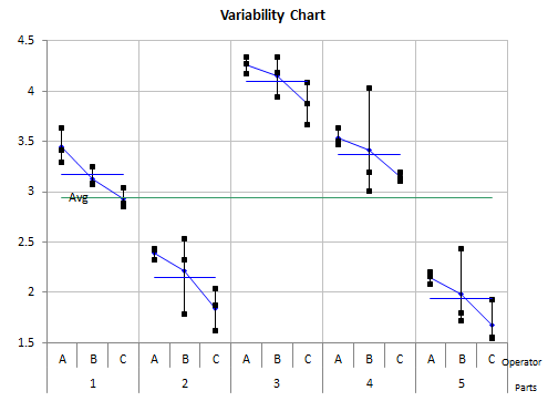
The variability chart below shows the results by part by operator.
Interaction Sum of Square and Degrees of Freedom
We will make use of the equality stated earlier to find the interaction sum of squares. This equality was:
SST = SS0 + SSP + SS0*P + SSE
SS0*P = SST– (SS0 + SSP + SSE)
SS0*P = 32.317 – (1.63 + 28.909 + 1.712)
SS0*P = 0.065
The same equality holds for the degrees of freedom:
df0*P = dfT – (df0 + dfP + dfE)
df0*P =44 – (2 + 4 + 30)
df0*P = 8
Summary
This is the first of a multi-part series on using ANOVA to analyze a Gage R&R study. It focused on providing a detailed explanation of how the calculations are done for the sum of squares and degrees of freedom. We will finish out the ANOVA table as well as complete the Gage R&R calculations in the coming issues.
Very well written post. It will be valuable to anybody who utilizes it, as well as myself. Keep doing what you are doing – for sure i will check out more posts.
Sum of squares for parts are wrong because, the upper limit for the summation should be n(number of parts) instead of k.
Thanks for catching that. It has been changed.
the formula to calculate the SSp has a term that must be (n*r) instead of (k*r)
I believe the formula is correct. It is measruing the sum of squares of the parts. k =number of operators and r = number of trials (replicates), so it gives 9 results per part.
Firstly thank you very much for this work, much appreciated!My quesiton would how you get from "Sum of Deviations" to "15(Sum of Deviations)" – for example the value for the operator is SS<sub>O</sub> = 1.6304 but the calculations seems to be missing in the math expression and the explanation:"n = 5 and r = 3, so there are 15 results for each operator" will just not match up for me.I would appreciate if you could explain the math a bit more in details – thanks in advance.
It appears I had the parts sum of squares in twice – for the parts and for the operators. Take a look at the equation SSo now. Thanks for pointing that out.
I am doing a Gauge R&R study for our test equipment.As we know, the %total variation is the sum of %variance contributed by part-to-part, operator and repeatability. The % total variation is always equal to 100%. In the other words, if the part-to-part variation is very big, then the %Gauge R&R(=%variance of operator+%variance of repeatibility) will be small and likely will pass the Gauge R&R. Is that true?If this is true, in order to pass the Gauge R&R we can select the big variance of the parts. Is that right thing to do?
Three methods for comparing results. One is to compare the gage variation to the variation of the parts used in the study. In this case, the parts should be selected to reflect the range of variation in the process. In other words, don't just take 10 parts off the line right in a row. You need to select the parts so they reflect the variation seen in the manufacturing process. This is the approach to take if you want the test method to be able to tell the differnce between parts (i.e., control the process).
The other two ways to determine the % gage R&R is to use an independent estimate of the process variation or to compare the results to the specification range. If you have an independent estimate of the process variation (e.g., from a control chart kept on the production process), the requirement for the parts spanning the production range is less critical. This is also true if you are comparing the results to the specification range. On the specs, in this case, you are just using the test to accept or reject parts.
Thank you so much for your clear explaination! I will try to compare the results to the specification range and see what is the different in the %gage R&R result then.
Hi Bill.Thanks for this example. My question is that having done a similar study using Minitab and excel, I get different results from the two methods. I have checked it with my colleagues and still its the same issue. Do you happen to know why that could be?Thanks
Hi David. Our SPC for Excel software gives the same results as Minitab. I assume you are doing this manually in Excel. Please send me the workbook and I will take a look at it. Send it to bill@www.spcforexcel.com
Muy bien!! Muchisimas gracias excelente explicación.
In the ANOVA Table for Gage R&R, Column F, all three items should be divided by the Mean Square (Equipment) MSe, not just the last one. Other Authorities use MSe as the divisior. MiniTab uses both MSe and MSo*p depending of an undisclosed calculation.
The table is correct if you keep the inteaction term in the model, which this article does. The part and operator F values are determined by dividing by MSo*p as shown in the table above. The F value for the interaction term is determined by dividing by MSE. Minitab does this as well.
If the interaction term in not significant and is removed from the model, then the F values for the parts and operators are determined by dividing MSE. This is also how Minitab handles it.
I have read your article on the topic Variable Gauge R & R study. 1 confusion is still running in my mind that how could be find if Instrument or Appraiser take wrong value(reading).
Not sure what you mean by wrong reading. A gage R&R is a study of variation. The equipment variation is a measure of the variation in the instrument. The operator variation is a measure of the variation in the operators. You can compare those two variances to see which is larger.
If %EV = 23.3 and AV = 25.3% then what it's meaning?
You appear to be looking at the average/range method. Please see this link:
https://www.spcforexcel.com/knowledge/measurement-systems-analysis/variable-measurement-systems-part-4-gage-rr
The equations are given there, e.g.
%EV = 100(EV/TV) = 100(0.217/0.9285) = 23.3%
% AV = 100(AV/TV) = 100(0.235/0.9285) = 25.3%
where TV is the total variation based onthe standard deviation (not recommended to use this method – use ANOVA or EMP.)
So it is telling you how much of the 6*standard deviation is taken up by the equipment variation and the appraiser variation.
Please describe briefly about NDC value. On what factors NDC depends? In what ways we can increase NDC value.
Please see this link for the definition of NDC:https://www.spcforexcel.com/knowledge/measurement-systems-analysis/variable-measurement-systems-part-4-gage-rrThe equation is give there, You improve NDC by improving the measurement system, decreaseing the Gage R&R variance.
Sir is it standard to arrange the data this way in order to obtain a Gage R&R via Anova method? Is it such that the software understands just this format?
When you run the ANOVA method with SPC for Excel, you select the number of operators, trials and parts. A template is then generated to fill to do the analysis. The software runs based on the tempalte design.
I am doing a gage r r analysis but the variance of error for each operator is different. Is my analysis valid? If not what can I do? If yes, how my interpretation of results is different from the typical gage r r analysis?
Hello. I need to see the data to see what is happening. Can you send it to me? bill@www.spcforexcel.com. Thanks
How do you conduct a R&R study? Is it done for any feature on the drawing? How do you select a dimension on which you conduct a R&R? Does it have to be done on all dimensions / features? If the R&R is done for a particular dimension and an instrument does it hold good for all other domensions if we are using the same instrument?SridharFrom Indiagnsridhar@gmail.com
Lots of questions. How do conduct a gage R&R is here:
https://www.spcforexcel.com/knowledge/measurement-systems-analysis/variable-measurement-systems-part-4-gage-rr
You can see all our SPC Knowledge Base articles on Measurement Systems Analysis here:
https://www.spcforexcel.com/spc-for-excel-publications-category#measurementSystemsAnalysis
You can do it on any feature; Select the key dimensions for the customer, just because one is good doesn't mean all are.
You can apply R&R only at primary data or it is possible to apply it for combination of data. e.g R&R for A & B but also R&R for the difference: A-B?Is it possible to get R&R<20% for A & B and R&R >20% for A-B?
Not 100% sure of what you are trying to it – but i imagine you can design an experiment to look at A&B and A-B. Not sure what hte possible outcomes are.