July 2021
(Note: all the previous SPC Knowledge Base in the control charts basics category are listed on the right-hand side. Select this link for information on the SPC for Excel software.)
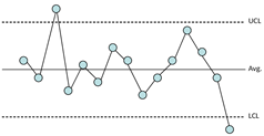
Obviously, you would like the control chart to signal that change on the next sample. Wouldn’t it be nice if that occurred each time there was a process shift? In the real world, unfortunately, that does not happen very often. Sometimes it can take two, three or ten or more samples for the control chart to show the process shift.
It depends primarily on the size of the shift you would like to detect. The larger the shift, the less samples on average it takes to detect the shift. The ability of a control chart to detect a shift is often characterized by the Average Run Length (ARL). This publication explores the ARL and what it means.
In this publication:
- Control Chart Review
- Selecting the Mathematical Model
- The Process Shift
- Calculating the ARL
- Summary
- Quick Links
Please feel free to leave a comment at the end of this publication. You can download a pdf copy at this link.
Control Chart Review
One purpose of a control chart is to monitor a process over time for signals that something has changed. It is the way the process communicates with you. By listening, the process – through the control chart – will tell you if everything is alright (just common causes of variation are present), or if there is a problem (a special cause of variation is present). You listen to the process by interpreting the control chart.
Suppose you are collecting data hourly on your process. The data for the last 20 hours is shown in Table 1.
Table 1: Data for the Last 20 Hours
| Sample | X | Sample | X | |
|---|---|---|---|---|
| 1 | 60.5 | 11 | 44.2 | |
| 2 | 33.5 | 12 | 55.4 | |
| 3 | 46.4 | 13 | 48.5 | |
| 4 | 51.3 | 14 | 37.5 | |
| 5 | 49.0 | 15 | 42.1 | |
| 6 | 46.5 | 16 | 47.8 | |
| 7 | 61.4 | 17 | 59.8 | |
| 8 | 52.7 | 18 | 47.5 | |
| 9 | 48.4 | 19 | 51.6 | |
| 10 | 48.3 | 20 | 79.2 |
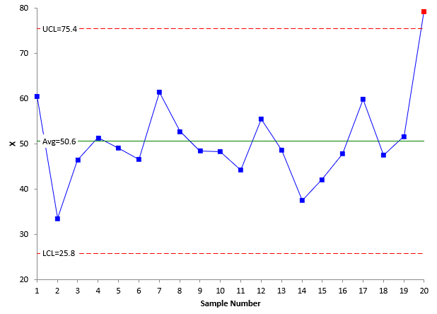
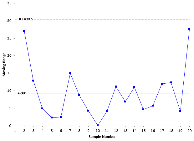
These data were used to construct the individuals control charts in Figures 1 and 2. Figure 1 is the X chart. Figure 2 is the moving range chart.
Figure 1: X Chart
Figure 2: Moving Range Chart
The last point on the X control chart is out of control – it is a point beyond the control limit. A special cause of variation is present. When an out of control point occurs, you are supposed to look for the root cause of it and eliminate that root cause, so it does not come back again in the process.
The reasons for out of control points are not always easy to find. Sometimes, a special cause is fleeting. It occurs for that point only and is gone by the time you look for the root cause. These are very hard to find. Sometimes it does represent a shift in the process. Something has changed in the process and may not change back until you find the root cause. Either way, the out of control point tells you something has changed significantly in the process.
The last point is out of control. Is this where the process change occurred? Maybe or maybe not. This is where the ARL comes in – it tells you the average run length before a process shift is detected. To do this, a mathematical model has to be selected.
Selecting the Mathematical Model
To calculate the ARL, you have to assume a mathematical model. For this publication, the normal distribution will be used. This does not mean that you must have a normal distribution to use a control chart – even the individuals control chart. A mathematical model is needed for the calculation of the ARL. We could use other distributions, such as the exponential distribution. But, for now, the assumption is that the mathematical model is the normal distribution.
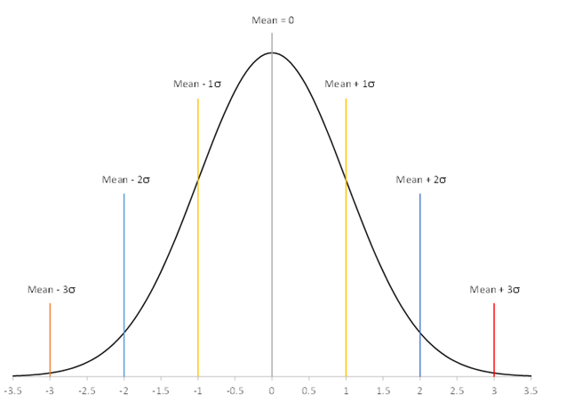
The standard normal distribution will be used. This normal distribution has a mean of 0 and a standard deviation of 1. It is shown in Figure 3.
Figure 3: Standard Normal Distribution
The normal distribution has the following characteristics:
- The shape of the distribution is determined by the mean and the standard deviation (0 and 1 respectively for the standard normal distribution)
- The highest point on the curve is the mean.
- The distribution is symmetrical about the mean.
- As you move away from the average, the points occur with less frequency.
- Most of the area under the curve (99.7%) lies between -3σ and +3σ of the mean.
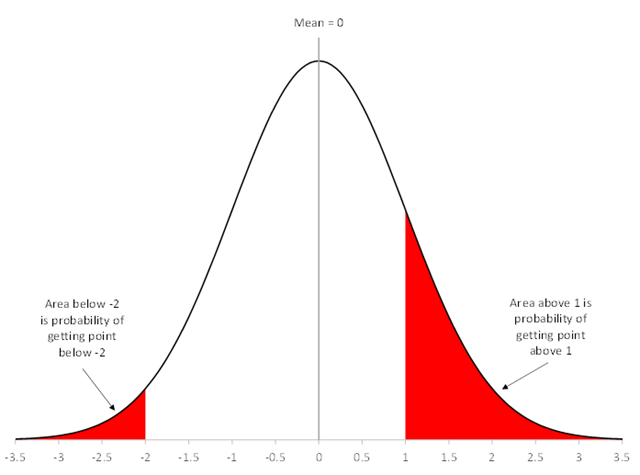
The standard normal distribution has the property that the area under the curve is equal to 1. You can use that knowledge to determine the probability that a point will be beyond a certain value, like the upper control limit (UCL) or below a certain value, like the lower control limit (LCL). This is shown in Figure 4.
Figure 4: Finding Area Under the Curve – Standard Normal Distribution
The red area on the left represents the area under the curve above 1σ. This is also the probability of getting a point above 1σ. Let “a” represent the area above 1c. You can calculate that area using Excel’s NORM.S.DIST function. The area above 1σ is given by:
a = 1 – NORM.S.DIST(1, True ) = 0.1587
There is a 15.87% probability of a point being beyond 1σ. You use the fact that the area under the curve is 1 when you are finding the area above a certain point using this Excel function.
The red area on the right represents the area under the curve below -2σ. The equation to find this area is:
a = NORM.S.DIST(2, TRUE) = 0.02275
There is a 2.28% probability of a point being below -2σ. You can find the area under the curve between -2σ and 1σ by adding the two areas above together and subtracting from 1.
The value of “a” plays an important role in determining the ARL.
The Process Shift
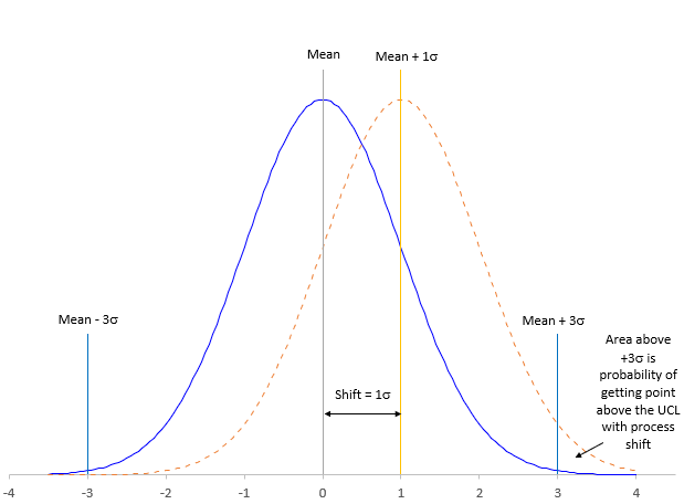
Suppose your process is in control. Suddenly, the process shifts by 1 sigma. The situation is depicted in Figure 5.
Figure 5: The Process Shift
The blue solid line is the original process (before the process shift occurred). The numbers on the x-axis represent sigma, e.g., – 1 means -1σ. The plot shows the mean +/- 3σ lines, which represent the location of the LCL and UCL.
The orange dotted line represents the process shift of 1 sigma. The new mean of the process is the mean + 1. The entire distribution has shifted to the right. The probability of getting a point beyond the existing UCL is the area under the curve greater than 2 for the shifted process.
For the shifted process, the mean + 2σ is the same as the mean + 3σ for the pre-shift process. The probability of getting a point beyond the mean + 2σ for the shifted process is:
a = 1 – NORM.S.DIST(2, TRUE) = .02275
With a process shift of 1 sigma, there is a 2.28% probability that the next point after the process shift will be beyond the existing UCL. The probability that the next point will be beyond the UCL is given by:
a(1 – a) = 0.02275(1 – 0.02275) = 0.02223
Adding these two numbers together gives the probability of detecting the process shift within the first two points: 0.02275 + 0.02223 = 0.04498. There is about a 4.5% probability of detecting the process shift within the first two points.
Let k = the number of points after the process shift. The probability (p) that a point will fall beyond the UCL with k points is given by:
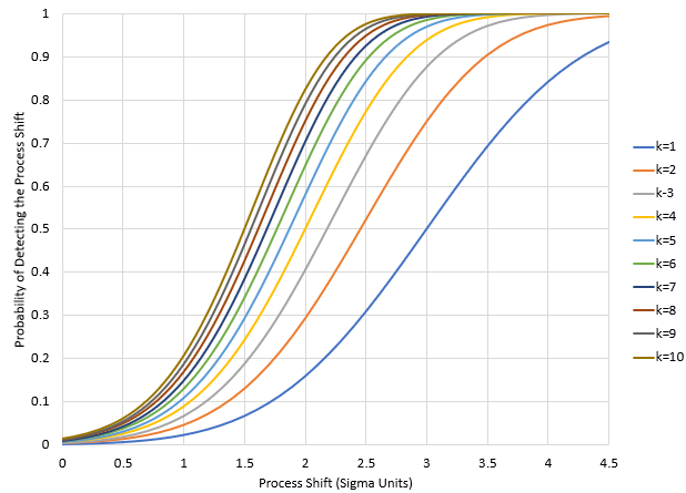
We can use the probability of detecting the process shift with the first point (a), the size of the shift and the number of observations (k) to build the “power function” curves for the individuals control chart. This chart is shown in Figure 6.
Figure 6: Power Function Curves for the X Control Chart for Points Beyond the Control Limits
The example above was a 1 sigma shift. You can see the first two points have a probability of about 0.045 from the graph. With 10 points, the probability of detecting the shift is only about 0.20 or 20%. You can confirm this with the equation from above:
1-(1-a)k=1-(1- .02275)10=0.2056
That is a lot of points before picking up the 1 sigma shift. This is why it is recommended you use other tests besides points beyond the control limits (e.g., zones tests) if you need to pick up smaller process shifts.
Suppose the process shift is 3 sigma to the right. In this case, the new process mean would be the same as the +3σ, the UCL for the pre-shift process. In this case, a = 0.5. This means that there is a 50% probability of detecting the process shift with the first point after the process shift; a 75% chance within the first two points and about 88% chance within the first three points. The larger the shift, the easier it is to detect using the points beyond the control limit test.
You can use these results to calculate the ARL.
Calculating the ARL
The average run length is calculated by multiplying each value of k by the probability of detecting the shift on the kth observation and then summing those products up. It is also given by the following:
Average Run Length (ARL) = 1/a
As shown above, a = 0.5 for the three sigma shift. Thus, the ARL for a three sigma shift is 1/0.5 = 2. This means, that on average, it will take 2 points to detect a 3 sigma process shift.
For a 1 sigma shift, a = 0.02275, so the ARL = 1/a = 1/.02275 = 44. This means, on average, it will take 44 points to detect a 1 sigma shift. A lot of points – again, a reason to use other out of control tests, such as the zone tests, to detect smaller process shifts.
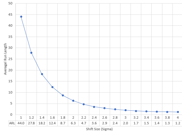
Figure 7 is a plot of the ARL versus various shift sizes for the X chart.
Figure 7: ARL versus Size Shift for the X Control Chart
You can see that ARL decreases as the size of the process shift increases. Of course, this is not surprising. But it does show the need to use the additional out of control tests to detect small process shifts more quickly.
Summary
Your process has an out of control point – a point beyond the control limit. The process may have shifted. When did this shift occur? At the out of control point? Or before? You really don’t know. The control chart has just detected it. How long will it take a control chart to detect the process shift as a signal? It depends on the size of the shift. The larger the shift, the easier it is to detect. The average run length (ARL) is a measure of how well a control chart detects the process shift. This publication examined the ARL for the X (individuals) control chart.

I belive thre is a typo error: the mshif is +1sigma and +2sigma.The following exerpt:”The probability of getting a point beyond the mean + 2σ for the shifted process is:a = 1 – NORM.S.DIST(2, TRUE) = .02275″is correct for +1sigma.
I believe the article is correct. If a process shifts +1 sigma, the "new" 2 sigma is where the "old" 3 sigma was. So, you are looking at the area above +2 sigma, which is 0.02275.
good
Thanks, good introduction to ARL