September 2012
 This month’s newsletter is the second in a multi-part series on using the ANOVA method for a Gage R&R study. This method simply uses analysis of variance to analyze the results of a gage R&R study instead of the classical average and range method. The two methods do not generate the same results, but they will (in most cases) be similar. With the ANOVA method, we will break down the variance into four components: parts, operators, interaction between parts and operators and the repeatability error due to the measurement system (or gage) itself.
The first part of this series focused on part of the ANOVA table. We took an in-depth look at how the sum of squares and degrees of freedom were determined. Many people do not understand how the calculations work and the information that is contained in the sum of squares and the degrees of freedom. In this issue we will complete the ANOVA table and show how to determine the % of total variance that is due to the measurement system (the % GRR).
In this issue:
- The Data
- The ANOVA Table for Gage R&R
- The ANOVA Table Results
- Expected Mean Squares
- The Variances of the Components
- The % Gage R&R
- Summary
- Quick Links
As always, please feel free to leave a comment at the bottom newsletter.
The Data
We are using the data from our December 2007 newsletter on the average and range method for Gage R&R. This newsletter also explains how to set up a gage R&R study. In this example, there were three operators who tested five parts three times. A partial picture of the Gage R&R design is shown below.
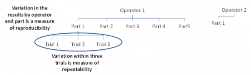
Operator 1 tested each 5 parts three times. In the figure above, you can see that Operator 1 has tested Part 1 three times. What are the sources of variation in these three trials? It is the measurement equipment itself. The operator is the same and the part is the same. The variation in these three trials is a measure of the repeatability. It is also called the equipment variation in Gage R&R studies or just with the “within” variation in ANOVA studies.
Operator 1 also runs Parts 2 through 5 three times each. The variation in those results includes the variation due to the parts as well as the equipment variation. Operator 2 and 3 also test the same 5 parts three times each. The variation in all results includes the equipment variation, the part variation, the operator variation and the interaction between operators and parts. An interaction can exist if the operator and parts are not independent. The variation due to operators is called the reproducibility. The data we are using are shown in the table below.
| Operator | Part | Results | ||
| A | 1 | 3.29 | 3.41 | 3.64 |
| 2 | 2.44 | 2.32 | 2.42 | |
| 3 | 4.34 | 4.17 | 4.27 | |
| 4 | 3.47 | 3.5 | 3.64 | |
| 5 | 2.2 | 2.08 | 2.16 | |
| B | 1 | 3.08 | 3.25 | 3.07 |
| 2 | 2.53 | 1.78 | 2.32 | |
| 3 | 4.19 | 3.94 | 4.34 | |
| 4 | 3.01 | 4.03 | 3.2 | |
| 5 | 2.44 | 1.8 | 1.72 | |
| C | 1 | 3.04 | 2.89 | 2.85 |
| 2 | 1.62 | 1.87 | 2.04 | |
| 3 | 3.88 | 4.09 | 3.67 | |
| 4 | 3.14 | 3.2 | 3.11 | |
| 5 | 1.54 | 1.93 | 1.55 | |
The ANOVA Table for Gage R&R
In most cases, you will use computer software to do the calculations. Since this is a relatively simple Gage R&R, we will show how the calculations are done. This helps understand the process better. The software usually displays the results in an ANOVA table. The basic ANOVA table is shown in the table below for the following where k = number of operators, r = number of replications, and n= number of parts.
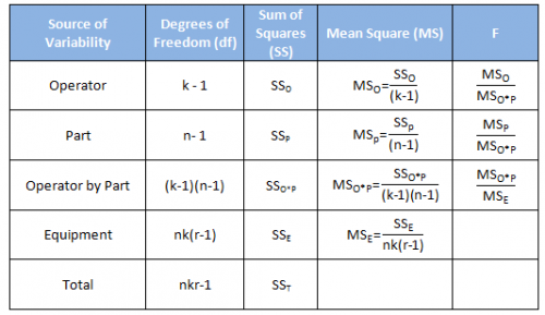
The first column is the source of variability. Remember that a Gage R&R study is a study of variation. There are five sources of variability in this ANOVA approach: the operator, the part, the interaction between the operator and part, the equipment and the total.
The second column is the degrees of freedom associated with the source of variation. The third column is the sum of squares. The calculations with these two columns were covered in the first part of this series.
The fourth column is the mean square associated with the source of variation. The mean square is the estimate of the variance for that source of variability (not necessarily by itself) based on the amount of data we have (the degrees of freedom). So, the mean square is the sum of squares divided by the degrees of freedom. We will use the mean square information to estimate the variance of each source of variation – this is the key to analyzing the Gage R&R results.
The fifth column is the F value. This is the statistic that is calculated to determine if the source of variability is statistically significant. It is based on the ratio of two variances (or mean squares in this case).
The ANOVA Table Results
The data was analyzed using the SPC for Excel software. The results for the ANOVA table are shown below.
| Source | df | SS | MS | F | p Value |
| Operator | 2 | 1.630 | 0.815 | 100.322 | 0.0000 |
| Part | 4 | 28.909 | 7.227 | 889.458 | 0.0000 |
| Operator by Part | 8 | 0.065 | 0.008 | 0.142 | 0.9964 |
| Equipment | 30 | 1.712 | 0.057 | ||
| Total | 44 | 32.317 |
Note that there is an additional column in this output – the p values. This is the column we want to examine first. If the p value is less than 0.05, it means that the source of variation has a significant impact on the results. As you can see in the table, the “operator by part” source is not significant. Its p value is 0.9964. Many software packages contain an option to remove the interaction if the p value is above a certain value – most often 0.25. In that case, the interaction is rolled into the equipment variation. We will keep it in the calculations here – though it has little impact since its mean square is so small.
The next column we want to look at is the mean square column. This column is an estimate of the variance due to the source of variation. So,
MSOperators = 0.815
MSParts = 7.227
MSOperators*Parts = 0.008
MSEquipment = 0.057
You might be tempted to assume, for example, that the variance due to the operators is 0.815. However, this would be wrong. There are other sources of variation present in all put one of these variances. We must use the Expected Mean Square to find out what other sources of variation are present. We will use σ2to denote a variance due to a single source.
Expected Mean Squares
As stated above, the mean square column contains a variance that is related to the source of variation in the first column. To find the variance of each source of variation, we have to use the expected mean square (EMS). The expected mean square represents the variance that the mean square column is estimating.
There are algorithms that allow you to generate the expected mean squares. This is beyond the scope of this newsletter. So, we will just present the expected mean squares.
Let’s start at the bottom with the equipment variation. This is really the within variation (also called error). It is the repeatability portion of the Gage R&R study. The expected mean square for equipment is the repeatability variance. The repeatability variance is the mean square of the equipment from the ANOVA table.
![]()
Now consider the interaction expected mean square which is given by:
![]()
Note that the EMS for the interaction tern contains the repeatability variance as well as the variance of the interaction between the operators and parts. This is what is estimated by the mean square of the interaction. The parts expected mean square is shown below.
![]()
Note that the EMS for parts contains the variances for repeatability, the interaction and parts. This is what is estimated by the mean square for parts. And last, the expected mean square for the operators is given by:
![]()
The EMS for operators contains the variances for repeatability, the interaction and operators. This is what the mean square for operators is estimating.
The Variances of the Components
We can solve the above equations for each individual σ2. Repeatability is already related directly to the mean square for equipment so we don’t need to do anything there. The other three can be solved as follows:

We can now do the calculations to estimate each of the variances.

Note that the value of the variance for the interaction between the operators and parts is actually negative. If this happens, the variance is simply set to zero.
% Gage R&R
The Measurement Systems Analysis manual published by AIAG (www.aiag.org) provides the following definition: The measurement system variation for repeatability and reproducibility (or GRR) is defined as the following:
GRR2=EV2 + AV2
where EV is the equipment variance and AV is the appraiser (or operator) variance. Thus:
![]()
The total variance is the sum of the components:
![]()
We can use the total variance to determine the % contribution of each source to the total variance. This is done by dividing the variance for each source by the total variance. For example, the % variation due to GRR is given by:
![]()
The results for all the sources of variation are shown in the table below.
| Source | Variance | % of Total Variance |
| GRR | 0.1109 | 12.14% |
| Equipment (Repeatability) | 0.0571 | 6.25% |
| Operators (Reproducibility) | 0.0538 | 5.89% |
| Interaction | 0.0000 | 0.00% |
| Parts | 0.8021 | 87.86% |
| Total | 0.9130 | 100.00% |
Based on this analysis, the measurement system is responsibility for 12.14% of the total variance. This may or may not be acceptable depending on the process and what your customer needs and wants. Note that this result is based on the total variance. It is very important that the parts you use in the Gage R&R study represent the range of values you will get from production.
One of the major problems people have with Gage R&R studies is selecting samples that do not truly reflect the range of production. If you have to do that, you can begin to look at how the results compare to specifications. We will take a look at that next month as we compare the ANOVA method to the Average and Range method for analyzing a Gage R&R experiment. You could also use a variance calculated directly from a month’s worth of production in place of the total variance in the analysis.
Summary
In this newsletter, we continued our exploration of the using ANOVA to analyze a Gage R&R experiment. We completed the ANOVA table, presented the expected mean squares and how to use those to estimate the variances of the components, and showed how to determine the %GRR as a percent of the total variance.
In the next newsletter, we will compare the ANOVA method to the Average and Range method for Gage R&R.
Anova Gage R&R process for attribute data?
HelloI am Venugopal from India. I am in Automotive field in Quality and i am also certified Six Sgima Black Belt from ASQ.Just to understand the concepts behind how minitab calculates all these, i went trough all the above articles series 1 to 3.Very intresting and detailed. Thanks for the same.I have some doubts on Expected mean Square variation. Can you throw some more details for this?ThanksVenugopalmail ID – vk5672@gmail.com91-9790888731
Hello,
What doubts do you have the EMS?
The denominator in the formula is r, which was explained as the number of replicates. number of replicates given was 3. But in the formula is filled in 5, which is the number of parts. What is right?
Hi Frank,
Good catch. The denominator is r = the number of replicates. So, it should be 3, not 5. I made the change. Note that the denominator for each EMS contains those not in the EMS. For example, the operator EMS denominator contains the number of parts times the number of replicates. So, the EMS for operators*parts contains the number of replicates.
For Simplicity , can we use Sum of Squares contribution to calculate Gage R and R. for example Can we say:Gage R&R ~ (SSo+SSo*p+SSe)/SSt
No, because the relationship is based on the variances, not the sum of squares. You use the EMS to find out how the mean squares can be used to determine the various variances.
As the equation shows GRR^2 = EV^2 + AV^2, wouldn't you need take the square root of 0.1109 to get GRR? In that case, the %GRR should be much higher.
The equation left off the squared. % GRR = GRR^2/TV^2/ Equation is corrected above.
I would expect for the equation for GRR^2 that the /sigma_Operators*Parts^2 would also contribute, since I think it is part of the appraiser variation. Well, in this case since interaction is small, it wouldn’t make a difference. But since you say you will include it… Am I right?
Not sure I understand the question but,the MS for Operators*Parts is like the MS for parts or operators by themselves.
Yes, you are correct! I was stuck on this for the longest time because the calculations I made did not match my data. That's when I noticed my /sigma_Operators*Parts^2 value is significant (as compared to the insignificance of this dataset) so I included it in the equation for GRR^2.
hi there, how would you calculate the variance of each component, the expected mean square, in stata?
I am not familiar with stata.
The results of GRR study changes if the piece that we want to measure is out of tolerance?
If you are using a historical standard deviation for the total variation, then the answer is no. If you are using the parts in the gage R&R to determine the total variation – and you substitute parts with mroe variaiton – then total variaiton will change.
The "% of Total Variance" in the final table sums up to 112,14 %. Probably shouldn't?
It sums to 100%. The Gage R&R (12.14) is broken in the two R components in the table. So you are double summing them when you get 112.14.
The articles are quiet interesting and detailed.Unfortunately all links given on the right of this webpage are available as pdfs for future reading. Is it possible to provide the same.SridharFrom Indiagnsridhar@gmail.com
Our older articles do have pdf downloads. Sorry. You may copy the webpage and paste it into Word though if you like.
Hi, at the ANOVA table resuts F.DIST gives a different result for the O*P p-value.<br />Is there an available way to calculate the p-value in the table? How was is done here?
The software uses FDIST. If you are using F.DIST, you have to use the following: 1 – F.Dist(.142, 8, 30, True).
Thank you very much for the analysis explanation. My statistics skills are not best. I would like to know if I can extract an uncertainty value range for my measuring system from the repeatability values. For example, the minimum uncertainty of a measurement is ± VALUE%
Yes, probable error is what you want to use most likely. Please see this article:
https://www.spcforexcel.com/knowledge/measurement-systems-analysis/probable-error-and-your-measurement-system
Hi, this two way ANOVA does not need need to meet any assumptions? I learned that a two way ANOVA needs to meet errors normality, variables independence and variance homogeneity. I have tested normality and the data is not normally distributed. This means this ANOVA results can not be trusted, right?
Measurement error is normally distributed. Not sure how you tested for normality. But I would not worry about that here.
I have made the non-parametric Lilliefors test. I have already checked it and with level of significance of 5% errors do not follow a normal curve. Can it be a problem or, for those cases of gage r&r this should not be important?
I would not worry about that with Gage R&R.
It seems like Sigma sq Parts formula in EMS is wrong. It should be MS Parts – Sigma 2 repeatability – r. Sigma sq Op x Parts / kr
Hello,
Not sure how you got that formula. I rechecked the formula in the publication and it appears to be correct.