October 2012
 This month’s newsletter is the third in a three-part series on using the ANOVA method for a Gage R&R study. This method uses analysis of variance to analyze the results of a Gage R&R study instead of the classical Average and Range Method
Many people refer to the AIAG’s Measurement Systems Analysis Manual (www.aiag.org) when doing Gage R&R studies. AIAG stands for Automotive Industry Action Group. For years, the most used method for Gage R&R was the Average and Range Method. This method calculates the % of the total variation that is due to the Gage R&R (repeatability and reproducibility). The total variation is based on the standard deviation.
Recently more people are beginning to prefer the ANOVA method for conducting Gage R&R studies. The ANOVA method includes the interaction between the operators (or appraisers) and the parts. ANOVA breaks down the variance into four components: parts, operators, interaction between parts and operators and the repeatability error due to the measurement system (or gage) itself. The interaction seldom is often insignificant and has little, if any, impact on the results.
The ANOVA method, however, allows you to estimate the variance of the components. If you base the % of total variation on the variance, instead of the standard deviation, you can get very different results – as we will show you in this newsletter. Which is the best method to use?
In this issue:
- Sources of Variation
- Example Data
- Results Using the ANOVA Method
- Removing the Interaction Term
- Standard Deviation and the ANOVA Method
- Comparison of Average/Range Method to ANOVA Method
- Which Should I Use?
- Quick Links
The first part of this series focused on part of the ANOVA table. We took an in-depth look at how the sum of squares and degrees of freedom were determined. Many people do not understand how the calculations work and the information that is contained in the sum of squares and the degrees of freedom. In the second part of this series we completed the ANOVA table and showed how to determine the % of total variance that is due to the measurement system or what is also called the % GRR.
We will start this newsletter with a review of the sources of variation in a process. This is followed by refreshing your memory with the data set we are using and the ANOVA results from the first and second part of this newsletter series. We will then look at how AIAG uses the standard deviation to estimate of the % GRR and how this differs from using the variance to perform the estimate of the % GRR. We will then compare the ANOVA method and the average and range method.
As always, please feel free to leave a comment.
Sources of Variation
 Suppose you are monitoring a process by pulling samples of the product at some regular interval and measuring one critical quality characteristic (X). Obviously, you will not always get the same result when measure for X. Why not? There are many sources of variation in the process. However, these sources can be grouped into three categories:
- variation due to the process itself
- variation due to sampling
- variation due to the measurement system
These three components of variation are related by the following:
σt2= σp2+ σs2+ σms2
where σt2is the total process variance; σp2is the process variance; σs2is the sampling variance and σms2is the measurement system variance. Note that the relationship is linear in terms of the variance (which is the square of the standard deviation), not the standard deviation.
For our purposes here, we will ignore the variance due to sampling (or more correctly, just include it as part of the process itself). However, for some processes, sampling variation can greatly impact the results. Thus, we will consider the total variance to be:
σt2= σp2+ σms2
Remember geometry? The right triangle? The Pythagorean Theorem? The above equation can be represented by the triangle below.
Figure 1: Sources of Variation
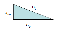
The total standard deviation, σt, for a measurement is equal to the length of the hypotenuse. The process standard deviation, σp, is equal to the length of one side of the triangle and the measurement system standard deviation, σms, is equal to the length of the remaining side.
You can easily see from this triangle what happens as the variation in the product and measurement system changes. If the product standard deviation is larger than the measurement standard deviation, it will have the larger impact on the total standard deviation. However, if the measurement standard deviation becomes too large, it will begin to have the largest impact.
Thus, the objective of improving a measurement system is to minimize the % variance due to the measurement system:
% Variance due to measurement system = 100(σms2/σt2)
In a Gage R&R study, you can break down σms2into its two components:
Repeatability is the ability of the measurement system to repeat the same measurements on the same sample under the same conditions. It represents an assessment of the ability to get the same measurement result each time.
Reproducibility is the ability of measurement system to return consistent measurements while varying the measurement conditions (different operators, different parts, etc.) It represents an assessment of the ability to reproduce the measurement of other operators.
Example Data
We are using the data from our December 2007 newsletter on the Average and Range Method for Gage R&R. In this example, there were three operators who tested five parts three times. A picture of part of the Gage R&R design is shown below.
Figure 2: Gage R&R Setup
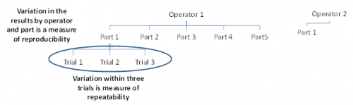
Operator 1 will test 5 parts three times each. In the figure above, you can see that Operator 1 has tested Part 1 three times. What are the sources of variation in these three trials? It is the measurement equipment itself. The operator is the same and the part is the same. The variation in these three trials is a measure of the repeatability. It is also called the equipment variation in Gage R&R studies or the “within” variation in ANOVA studies.
Operator 1 also runs Parts 2 through 5 three times each. The variation in those results includes the variation due to the parts as well as the equipment variation. Operator 2 and 3 also test the same 5 parts three times each. The variation in all results includes the equipment variation, the part variation, the operator variation and the interaction between operators and parts. The variation in all results is the reproducibility.
The data from the December 2007 newsletter are shown in the table below.
Table 1: The Gage R&R Data
| Operator | Part | Results | ||
| A | 1 | 3.29 | 3.41 | 3.64 |
| 2 | 2.44 | 2.32 | 2.42 | |
| 3 | 4.34 | 4.17 | 4.27 | |
| 4 | 3.47 | 3.5 | 3.64 | |
| 5 | 2.2 | 2.08 | 2.16 | |
| B | 1 | 3.08 | 3.25 | 3.07 |
| 2 | 2.53 | 1.78 | 2.32 | |
| 3 | 4.19 | 3.94 | 4.34 | |
| 4 | 3.01 | 4.03 | 3.2 | |
| 5 | 2.44 | 1.8 | 1.72 | |
| C | 1 | 3.04 | 2.89 | 2.85 |
| 2 | 1.62 | 1.87 | 2.04 | |
| 3 | 3.88 | 4.09 | 3.67 | |
| 4 | 3.14 | 3.2 | 3.11 | |
| 5 | 1.54 | 1.93 | 1.55 | |
The operator is listed in first column and the part numbers in the second column. The next three columns contain the results of the three trials for that operator and part number. For example, the three trial results for Operator A and Part 1 are 3.29, 3.41 and 3.64.
Results Using the ANOVA Method
The data was analyzed using the SPC for Excel software. The ANOVA table is shown below.
Table 2: The ANOVA Results
| Source | df | SS | MS | F | p Value |
| Operator | 2 | 1.630 | 0.815 | 100.322 | 0.0000 |
| Part | 4 | 28.909 | 7.227 | 889.458 | 0.0000 |
| Operator by Part | 8 | 0.065 | 0.008 | 0.142 | 0.9964 |
| Equipment | 30 | 1.712 | 0.057 | ||
| Total | 44 | 32.317 |
As you can see in the table, the “operator by part” source is not significant. Its p value is 0.9964. Many software packages contain an option to remove the interaction if the p value is above a certain value – most often 0.25. In that case, the interaction is rolled into the equipment variation. We kept it in the calculations in Part 2 – though it has little impact since its mean square is so small.
The results for all the sources of variation are shown in the table below. The calculations are given in detail in Part 2 of this newsletter series. The calculations show how to estimate the variances in the table below. Then to find the contribution to % of total variance, you simply divide the estimate of the variance for the source by the total variance. You can see from the results, that the Gage R&R is responsible for 12.14% of the total variance.
Table 3: Contribution to % Total Variance Including the Interaction
| Source | Variance | % of Total Variance |
| GRR | 0.1109 | 12.14% |
| Equipment (Repeatability) | 0.0571 | 6.25% |
| Operators (Reproducibility) | 0.0538 | 5.89% |
| Interaction | 0.0000 | 0.00% |
| Parts | 0.8021 | 87.86% |
| Total | 0.9130 | 100.00% |
The % GRR given in Table 3 will not be the same as the one you get from the Average and Range Method – as we will show below. The approach above uses the total variance to compare the each source of variation while the Average and Range Method uses the total standard deviation.
Removing the Interaction
As mentioned above, many software packages have the option to remove the interaction term if alpha is above a certain value (usually 0.25). This means that if the p value for the interaction term in the ANOVA table is greater than this value, the interaction is considered to be zero and is removed. As you can see in the ANOVA table above, the p value for the interaction term is 0.9964. If this term is removed, the contribution to the % of total variance changes slightly as seen in the table below.
Table 4: Contribution to % Total Variance Without the Interaction
|
Source of Variation |
Estimate of Variance |
% of Total Variance |
|
GRR |
0.0980 |
10.94% |
|
Equipment (Repeatability) |
0.0468 |
5.22% |
|
Operator (Reproducibility) |
0.0512 |
5.72% |
|
Part |
0.798 |
89.06% |
|
Total Variation |
0.896 |
100.00% |
If the interaction is significant, removing it will have a much greater impact on the result. You should not remove the interaction if it is significant.
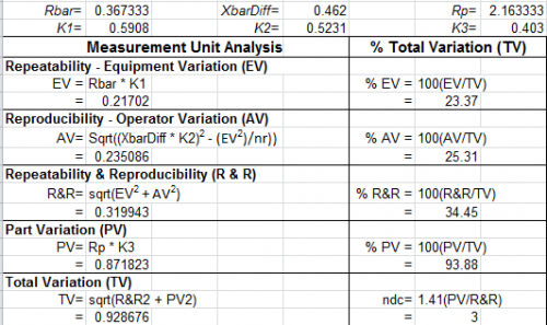
Standard Deviation and the ANOVA Method
You should note that the results in the table above are based on the contribution of each source to the % of total variance. AIAG’s average and range method bases the results on standard deviation, not the variance. This is one of the major issues some folks have with the average and range method – the standard deviations are not additive – like the variances are.
However, AIAG says that “the standard deviation is easier to interpret than variance because it has the same unit of measure as the original observation” (page 196, 4th edition). In fact, AIAG includes the standard deviation in the ANOVA output. The output looks something like the following:
Table 5: % of Total Variation Based on Standard Deviation
| Source of Variation | Estimate of Variance | Std. Dev. | 6 * Std. Dev. | % Total Variation | % Contribution | |
| Equipment | 0.0468 | 0.216 | EV = | 1.298 | 22.85% | 5.22% |
| Operator | 0.0512 | 0.226 | AV = | 1.358 | 23.91% | 5.72% |
| Interaction | 0.0000 | 0.000 | INT = | 0.000 | 0.00% | 0.00% |
| GRR | 0.0980 | 0.313 | GRR = | 1.878 | 33.07% | 10.94% |
| Part | 0.7978 | 0.893 | PV = | 5.359 | 94.37% | 89.06% |
| Total Variation | 0.8958 | 0.946 | TV = | 5.679 | 100.00% | |
The table above does not include the interaction term since it is insignificant. The first column is the source of the variation – such as equipment. The second column is the estimate of the variance from the ANOVA results (see Part 2 of this series for how to estimate these). These values are the same as those in table 4. The third column is the standard deviation. This is simply the square root each of the variances.
The fourth column multiplies the standard deviation by a “sigma” multiplier. In the past, 5.15 was used, but the more recent editions of the Measurement Systems Analysis manual uses 6. This gives a spread of the results for each source of variation – in this case 6 sigma. In the table above, EV = equipment variability, AV = the appraiser (or operator variability), PV = the part variation and TV = the total variation.
The fifth column is the % of total variation. This is simply each source of variation’s six sigma spread divided by the total six sigma spread. So,
GRR % of Total Variation = 1.878/5.679 = 33%
The sixth column is the % of total variance for each source from the ANOVA analysis (Table4). You can see that the results are considerably different depending on the approach. Note that AIAG refers to this column as % contribution – but it is the % of total variance.
Why the large difference when looking at the % of total variation or the % of total variance? It is because the variances are additive and the standard deviations are not.
σTotal2= σEquipment2+ σOperators2+ σParts2
σTotal≠ σEquipment+ σOperators+ σParts
What this means is that when you add up the contribution of each source to the total variance, you will get 100%. However, when you add up the contribution to each source to the total variation (based on the standard deviation), you will not get 100%. In fact, when using the standard deviation, the % of total variation never add to 100. The table below shows the results for the data we are looking at.
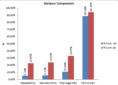
Table 6: Comparing % of Total Variation and % of Total Variance
|
Source of Variation |
% of Total Variation |
% of Total Variance |
|
GRR |
33.07% |
10.94% |
|
Equipment |
22.85% |
5.22% |
|
Operator |
23.91% |
5.72% |
|
Part |
94.37% |
89.06% |
|
Sum of GRR+Part |
127.45% |
100.00% |
Figure 3 shows the percentages in graphical form. There is a significant difference between using the % of total variation or the % of total variance.
Figure 3: Comparing % of Total Variation and % of Total Variance
Comparison of Average/Range Method to ANOVA Method
The average and range method described in an earlier newsletter. The output from the SPC for Excel software is shown below for the average and range method.
Table 7: GRR Based on Average and Range Method
The values for EV, AV, R&R, PV and TV are standard deviations determined using the Average and Range Method. You can see that the standard deviations and % of total variation given in this table are similar to the results from the ANOVA that are based on using the standard deviation. This is shown in Table 8 below. Thus, there is really no difference between the Average and Range Method and the ANOVA method based on AIAG’s approach of using the standard deviation.
Table 8: Comparison of Average and Range Method with the ANOVA Method
|
Source of Variation |
Std. Dev. from Average & Range Method |
% of Total Variation from Average & Range Method |
Std. Dev. From ANOVA |
% Total Variation from ANOVA |
|
GRR |
0.32 |
34.45 |
0.313 |
33.07 |
|
Equipment |
0.217 |
23.37 |
0.216 |
22.85 |
|
Operator |
0.235 |
25.31 |
0.226 |
23.91 |
|
Part |
0.872 |
93.88 |
0.893 |
94.37 |
|
Total Variation |
0.929 |
0.946 |
|
So, the results from the average and range method are very similar to the ANOVA method. The major question that should be asked is should I be basing the results on the standard deviation or on the variance?
Which Should I Use?
The question is not if you should use the ANOVA method or the Average and Range method for a Gage R&R study. Use whatever the customer wants you to. You will get pretty much the same results. The real question is: Do I base the results on the % of total variation (based on the standard deviation) or on the % of the total variance? I think it should be % of total variance. Variances are additive. The standard deviation is not. Our November 2009 newsletter took a look at how to evaluate a measurement system using control charts and the % of total variance due to the measurement system. We compared the results to the Discrimination Ratio discussed by Dr. Don Wheeler. We found that the % of total variance approach matched well. We defined a good measurement system as the following:
A good measurement system should not be responsible for more than 10% of the total variance.
If you have the option, go with the % of total variance.
Even AIAG in latest MSA versions (3 and 4) promotes the Anova method over the range method, and in semiconductor industry we adopted Anova method in 90's as it gave better insight. Nice newsletter overview of issues. JMP software recent versions have AIAG methods and Wheeler EMP methods, and appropriate graphs for each. The old excel spreadsheets with range method only are dying out slowly. With modern automated gages, no operator error is seen in many studies (other than gross errors like selection of wrong gage recipe, or mangling of parts being sampled.). So instead of %R&R with operators for reproducibility, we use multiple gages for studying matching of gages.That leads to some interesting economic issues of using frequent calibrations, vs offsets based on "golden gauge" with "golden parts" which can be a long story. MSA is a deep rathole to try to cover generically with any canned routine. NIST uncertainty methods are a parallel (not replacement) toolset that could be covered in future newsletters.
Great text, thank you so much for the insight.Small correction needed: the formula used for demonstrating that standard deviations are not addiditive still has a "squared" symbol on the standard deviation total.
Thanks for catching that. Proof once again that 100% inspection does not prevent defects. I corrected that text.
In Table 1, the final value is shown as 1.5. On another page, the value is shown as 1.55. Run ANOVA on the data in this page and you'll get different results from what is shown here. Run ANOVA where the final value is 1.55 and you'll get the results shown in this page.
Thanks Joe. I corrected the last value to be 1.55 as it should be.
Hi, I would like to ask, how I could calculate Estimate of Variance for Equipment (0,0468), Operator (0,0512) and Part (0,0512), when I remove the interaction. In part 2 it is written, that the interaction is rolled into the equipment variation, but I can´t get the mentioned values for Estimate of Variance. Could you help?
You use the expected mean square equations that are given in Part 2. What values are you getting?
Thanks a lot, now is clear for me
Hi, I have another question about calculation. In these articles there is mentioned p value calculated by software. It is possible to calculate this item without using of special software? I tried to use f.dist.rt function from excel. For p value – Operator by Part – I use =F.DIST.RT(0,43;8;30) with result 0,9964. It is my calculation ok? If yes, how I can set the degrees of freedom for calculation of other p values (Operator, Part)? Could you help also with this? Thanks
You can use FDIST(F value, degrees of freedom in numerator, degrees of freedom in denominator). F value for operator by part is determined by MS Operator by part/MS Equipment so FDIST(0.142, 8, 30). F for part by MS Part/MS Operator by Part so FDIST(889.458, 4, 8). F for Operator by MS Operator/MS Operator by Part so FDIST(100.322, 2, 8)
Thanks
Hi Bill! I'm from Brazil and I read all about R&R Anova here. I didn't understand when you said "You use the expected mean square equations that are given in Part 2". It's mean that I should to use all the equations, as they are, without the source Operators*parts? Because I tried but didn't work. I can't found 0.0468 for the Estimate of Variance for Equipment. Obrigado!
I’m unable to understand how these numbers, Estimate of Variance for Equipment (0,0468), Operator (0,0512) and Part (0,0512 were derived in Table 4. Referring to Part 2, the interaction is already 0.000 in the equations. So the results would be same as Table 3, isn’t it? What am I missing?
Look at Table 2. You can see the interaction term in that table. It has 8 degrees of freedom and the SS is 0.065. Since the interaction is not significant and is removed, these values are added to the values for the equipment. This changes the ANOVA table (not shown in the publication). This changes the values used to caculate the % of variance. Please let me know if you need more information.
Bill
Yes, I also am having trouble following how the values in Table 4 are derived. Is it possible to explain that process in more detail?
The operator*Part intereaction is not included the analysis, it becomes part of the equipment vartiation.
Dear Bill,Could you please share any example where GRR is applied for two same machines with N number of Operators and K number of Parts. Any LINK will also work.Thanks & RegardsAshok
I would take a look at Two-Factor EMP studies in Dr. Wheeler's book Evaluating the Measurement Process (EMP III). He has a chapter that shows how to analyze a test method used on two different instruments. Now, if you just want to compare the two instruments, you can use the two instruments in place of appraisers and do a normal Gage R&R Analysis.
i need to find the value of standards (k1,k2) if i would take the trial by using 4 operators and 5 trials
How many parts are you using?
Hello, Bill! I think my question is probably foolish but it haunts my mind for a couple of months. Why total variation calculated by ANOVA (0.896) differs from sample variance (0.735)? Is there some relation between them?
Hello, it is not a foolish question at all. It is because of this is a designed experiement where you replicate things – same operator testing same part multiple times. So, the the total variance calculated by ANOVA is different from the sample variance. If you don't worry abou the operators and simply put the results in a table by part number and run the ANOVA in excel, you will see that the total variance from ANOVA is the sample variance – that is because you are not worried about anything but the part. Hope this helps.
Does anybody know why only a Part-Operator interaction is included? Are the Equipment-Part and Equipment-Appraiser interactions assumed to be zero or am I misunderstanding something fundamental about ANOVA GRR Analysis?
in the MSA where I find a table where it indicates the% Study Var and% Tolerance of acceptable of the Anova R&R study?
Please see this link: https://www.spcforexcel.com/knowledge/measurement-systems-analysis/acceptance-criteria-for-MSA