November 2020
(Note: all the previous SPC Knowledge Base in the measurement systems analysis category are listed on the right-hand side. Select this link for information on the SPC for Excel software.)

Do you have to improve the measurement system? No, not necessarily. A measurement system that is responsible for 50% of the total process variance is still very useful in detecting process signals on a control chart.
This months’ publication does a simple simulation to understand how increasing measurement error impacts the ability of a control chart to see a signal. We begin with a perfect measurement system – one with no variation at all. The ability of a control chart to pick up shifts of 1 to 5 sigma is shown. Measurement error is then added to the simulation to show the impact on the control chart’s ability to detect these shifts. The results may well surprise you.
In this publication:
- Introduction
- Relationship between Total, Product and Measurement Process Variation
- Intraclass Correlation Coefficient
- Simulating the Product and Measurement Error
- Product Data with No Measurement Error
- Product Data with Measurement Error
- The Four Classes of Monitors
- Summary
- Quick Links
You may download a pdf copy of this publication at this link. Please feel free to leave a comment at the end of the publication.
Introduction
Measurements are used to determine if we are improving, staying the same, or getting worse. We hope the measurement system gives us a signal if there has been a change in the process. This means that we hope the measurement system does not have too much variation that masks the signal that something has changed.
The most commonly used variable to see if our measurement system is useful is the % of total variance due to the measurement system. Unfortunately, it is too often compared to arbitrary guidelines, such as those from the Automotive Industry Action Group (AIAG). These guidelines are:
- If the % Gage R&R is under 10%, the measurement system is generally considered to be an adequate measurement system.
- If the % Gage R&R is between 10 % to 30%, the measurement system may be acceptable for some applications.
- If the % Gage R&R is over 30%, the measurement system is considered to be unacceptable.
These guidelines are based on using the standard deviation, not the variance. If you are using variance, like in an ANOVA Gage R&R, you square the numbers above. So, if the % Gage R&R is over 30%, this corresponds to 0.3 x 0.3 = 0.09 = 9% of the total variance. This says that if the measurement system is responsible for more than 9% of the total variance then the measurement system is considered to be unacceptable. This is NOT the way to look at results.
There is a much better way. That way is the system developed by Dr. Donald Wheeler in his Evaluating the Measurement Process procedures, that divides a measurement system into four categories: – First Class monitors, Second Class monitors, Third Class monitors and Fourth Class monitors. These categories give insight into the puzzle that is our measurement system. This publication examines one part of Dr. Wheeler’s classification scheme: how much the measurement system reduces a signal from the process.
For more information on the criteria for an acceptable measurement system, please see our SPC Knowledge Base article “Acceptance Criteria for Measurement System Analysis“.
Relationship between Total, Product and Measurement Process Variation
You take a sample from your process. You test that sample using your measurement system. You get a result (X1). You take another sample and test that sample. You get another result (X2). Usually X1 does not equal X2. What are in these results? Two major components are present in each result: the variation in the product itself and the variation in the measurement system.
The basic equation describing the relationship between the total variance, the product variance and the measurement system variance is given below.
σx2= σp2+σe2
where σx2= total variance of the product measurements, σp2= the variance of the product, and σe2= the variance of the measurement system.
We will use the ratio of the product variance to the total variance to define the “Intraclass Correlation Coefficient.” This is the variable that Dr. Wheeler uses to define how “useful” a measurement system is. It is directly related to the % of the total variance due to the measurement system.
Intraclass Correlation Coefficient
The Intraclass Correlation Coefficient is simply the ratio of the product variance to the total variance and is denoted by ρ:
ρ= (σp2/(σx2)
This is simply the % of the total variance that is due to the product variance. Remembering the basic equation above, then 1 – ρ is the % of the total variance that is due to the measurement system. This is essentially what we look at in ANOVA Gage R&R analysis.
% of total variance due to the measurement system = σe2=1 – ρ = 1 -(σp2/(σx2)
Simulating the Product and Measurement Error
A simple simulation is used to determine the effect of the measurement error on the ability of a control chart to detect a process change. This simulation is based on the one given by Dr. Wheeler in his book EMP III: Evaluating the Measurement Process & Using Imperfect Data (www.spcpress.com). It is assumed that the product (P) and the measurement error (E) are both normal distributions with a mean = 0 and a standard deviation = 1. The first simulation below assumes there is no measurement error – we have a perfect measurement system. 100 random numbers are generated for the product. This was done using the SPC for Excel software random number generator.
The individuals control chart is used to analyze the results. Only the X control chart is used. The X control chart is then produced for these 100 points for the product, and the control limits set based on the first 50 points. The control charts in this publication were produced using the SPC for Excel software.
Product shifts are then produced in the data for points 51 through 100. Product shifts of 1, 2, 3, 4 and 5 sigma are introduced – ten points for each. These shifts represent signals in the process. The X control chart is redrawn with these shifts and the ability of the control chart to detect signals is then analyzed.
Next, measurement error is introduced. In the simulation below, the measurement system variance is the same as the product variation; so, 50% of the total variance is due to the measurement system. 100 points are randomly generated for the measurement error. This measurement error is added to the product results (X = P + E) and the resulting X control chart analyzed. The shifts are then added. The X control chart is redrawn with the shifts and the ability of the control chart to detect signals with the added measurement error is analyzed.
The workbook with all the data used can be downloaded here.
Product Data with No Measurement Error
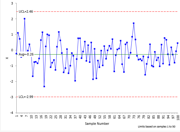
Figure 1 shows the product data with the control limits set based on the first 50 samples. This represents the case where the measurement error is 0.
Figure 1: Product Data (No Measurement Error)
If the simulation were perfect, the X control chart would have an average of 0 and a lower control limit (LCL) of -3 and an upper control limit (UCL) of 3. The average, based on the first 50 points, is -0.26 with a LCL = -2.99 and UCL = 2.46. The estimated value of sigma from the average moving range is 0.91. The average and standard deviation of the simulated data are close to the theoretical values.
The X control chart in Figure 1 is in statistical control. There are no points beyond the control limits and no patterns in the data.
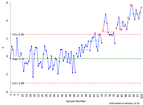
The next step is to add the signals to the data. This is done by simply adding a shift to each set of ten points after point 50. For points 51 to 60, a 1 sigma shift is added; points 61 to 70, a 2 sigma shift is added; points 71 to 80, a 3 sigma shift is added; points 81 to 90, a 4 sigma shift is added, and points 91 to 100, a 5 sigma shift is added. Each sigma shift is 1 (the theoretical standard deviation). The X control chart with the shifts added is shown in Figure 2.
Figure 2: Product Data (No Measurement Error) with Shifts Added
The short, horizontal lines represent the sigma shifts, the average plus the shift. As you can see, the 2 to five sigma shifts are picked up quickly as points beyond the control limits (in red). The one sigma shift is picked up as a run above the average – all ten points are above the average. The X control chart with no measurement error picks up the shifts in the process. Now, what happens if we add in measurement error? A lot of measurement error.
Product Data with Measurement Error
The X control chart above has no measurement error. Introducing measurement error will widen the control limits. This has the effect of lessening the signals seen on the chart. You cannot prevent that. To demonstrate what happens, we will add measurement error that is the same as the product variance. This means that the measurement system will be responsible for 50% of the total process variance – this can’t be a good measurement system. Can it?
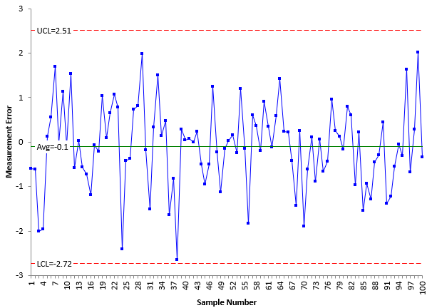
To generate the measurement error, 100 random points from a normal distribution with mean = 0 and standard deviation = 1 were generated. Figure 3 shows the X control chart for measurement error alone.
Figure 3: Measurement System Variation
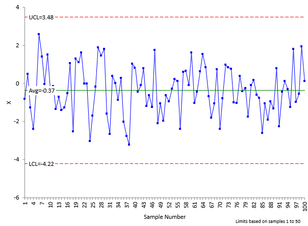
The average for the simulated data is -0.1. The estimated sigma from the average moving range is 0.87. The average and standard deviation are close to the theoretical values. This measurement error is added to the product data from Figure 1 and the control limits set for the first 50 samples. The resulting X control chart is shown in Figure 4.
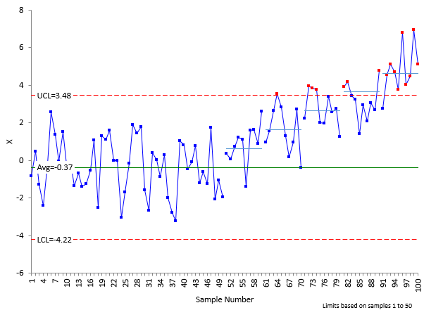
Figure 4: Product Data Plus Measurement Error Added
Compare the control limits in Figure 1 to Figure 4. You will see that the control limits in Figure 4 are wider. This is the effect of adding in measurement error. Figure 5 shows the impact of adding the 1 to 5 sigma shifts.
Figure 5: Product Data Plus Measurement Error Added with Shifts
What does this measurement system pick up? It does not pick up the one sigma shift within 10 samples (but most likely will soon with a run above the average) but it does pick up the 2 to 5 sigma shifts as points beyond the control limits.
What? A measurement system that is responsible for 50% of the total variance can do that? This measurement system is more than capable of catching major shifts quickly in the process. It seems acceptable to me. This is one advantage that the EMP classification scheme has over the other methods. It is based on what the measurement system can do and does not judge the measurement system against arbitrary guidelines.
Should you improve the measurement system? You should always work on continuous improvement. But if the cost to improve this measurement system is very large – or if there are higher priority items – then this measurement system is fine for now. Let’s look briefly at the classes of monitors.
The Four Classes of Monitors
Dr. Wheeler’s four classes of monitors are summarized in Table 1 below.
Table 1: The Four Classes of Process Monitors
| INTRACLASS COEFFICIENT | TYPE OF MONITOR | REDUCTION OF PROCESS SIGNAL | CHANCE OF DETECTING ± 3 STD. ERROR SHIFT | ABILITY TO TRACK PROCESS IMPROVEMENTS |
|---|---|---|---|---|
| 0.8 to 1.0 | First Class | Less than 10% | More than 99% with Rule 1 | Up to Cp80 |
| 0.5 to 0.8 | Second Class | From 10% to 30% | More than 88% with Rule 1 | Up to Cp50 |
| 0.2 to 0.5 | Third Class | From 30% to 55% | More than 91% with Rules 1, 2, 3 and 4 | Up to Cp20 |
| 0.0 to 0.2 | Fourth Class | More than 55% | Rapidly Vanishing | Unable to Track |
The first column lists the value of the Intraclass Correlation Coefficient. Remember that the % of total variance due to the measurement system is 1 – ?. A First Class Monitor has a? of 0.8 to 1.0 (80% to 100%). This corresponds to 0 to 20% for the % of total variance due to the measurement system. A First Class monitor is very good – but already fails the AIAG guideline since the % of total variance due to the measurement system could be greater than 9%.
The third column shows how much of a reduction in a process signal there is. The First Class monitor has less than a 10% reduction in process signal while a Fourth Class monitor has more than a 55% reduction in process signal. Our example was borderline between a Second and Third class monitor. But still has a great chance at picking up shifts in the process, particularly if you use the Western Electric zone tests:
- Rule 1: a point is beyond the lower or upper control limit
- Rule 2: two out of three consecutive points on the same side of the average are more than two standard deviations away from the average
- Rule 3: four out of five consecutive points on the same side of the average are more than one standard deviation away from the average
- Rule 4: Eight consecutive points are above or below the average
Note that the First and Second Class monitors detect Rule 1 very well. Once you reach a Third Class monitor, you need to apply all four rules to get the chance of detecting the shift high. Fourth Class monitors are not good at detecting any shifts essentially.
The fifth column describes the monitor’s ability to track process improvements. This is something we don’t think about too much. This last column describes how much process improvement you can have until the measurement system moves from one class to another.
For more information on the classes of monitors, please see our SPC Knowledge Base article “Evaluating the Measurement Process, Part 1.”
Summary
This month’s publication examined how the measurement system impacts a control chart’s ability to detect process signals – when the process has changed. A simple simulation was run that showed how this ability changes from a measurement system with no variation to one that is responsible for 50% of the total variance. Even with this amount of measurement system variation, the control chart was still able to pick up the shifts of 1 to 5 sigma. Dr. Wheeler’s monitor classification scheme presents a great method of determining how useful a measurement system is. This is the way you should classify your measurement systems.
