June 2019
(Note: all the previous SPC Knowledge Base in the measurement systems analysis category are listed on the right-hand side. Select this link for information on the SPC for Excel software.)

Dr. Donald Wheeler, over the years, has developed a process called Evaluating the Measurement Process (EMP). EMP consists of multiple techniques to evaluate a measurement process. One of those techniques is called the Short EMP Study. The Short EMP Study is the topic of this month’s publication.
In this issue:
- An Introduction to the Short EMP Study
- Example Data
- R Control Chart Results
- X Control Chart Results
- Relationship between Total, Product and Measurement Variation
- Other Insights for the EMP Short Study
- Summary
- SPC for Excel Version 6 is Now Available!
- Quick Links
Please feel free to leave a comment at the end of this publication. You can also download a copy of this publication at this link.
An Introduction to the Short EMP Study
The Short EMP study is a study where one operator runs multiple parts multiple times – like a Gage R&R analysis but with only one operator. For example, one operator might measure 10 parts 3 times each. The interesting thing about this approach is that it provides a picture of whether the measurement system can tell the difference between the parts used in the study.
The results are then analyzed using a X-R control chart. Subgroups are formed by combining the repeated results for one part. For example, subgroup 1 contains the three results when part 1 was run; subgroup 2 contains the three results when part 2 was run, etc. The average and range of each subgroup is calculated, and the results are then plotted on the X-R control chart. The resulting charts give you interesting insights into your measurement process. An example of the Short EMP Study is given below.
Example Data
Suppose you take 10 parts from your process and select them in such a way that they represent the variation that exists in the process. You measure each part for a given quality characteristic. The data generated are shown in Table 1.
Table 1: Short EMP Study Data
| Subgroup Number | X1 | X2 | X3 |
|---|---|---|---|
| 1 | 11.46 | 11.26 | 10.67 |
| 2 | 10.01 | 9.33 | 9.01 |
| 3 | 11.55 | 11.51 | 11.75 |
| 4 | 12.28 | 12.63 | 12.55 |
| 5 | 10.18 | 9.96 | 9.95 |
| 6 | 12.01 | 12.51 | 12.49 |
| 7 | 10.23 | 10.79 | 10.71 |
| 8 | 11.11 | 10.84 | 10.72 |
| 9 | 11.05 | 11.10 | 11.10 |
| 10 | 12.80 | 12.41 | 12.02 |
In this example, part 1 was measured three times. Subgroup 1 consists of those results: 11.46, 11.26 and 10.67. The other subgroups are formed in the same manner – from the three results for each part.
There are two subgroup results that we will analyze: one is the range within the subgroup, which we will analyze using the range control chart, and the other is the subgroup average, which we will analyze using the X control chart.
R Control Chart Results
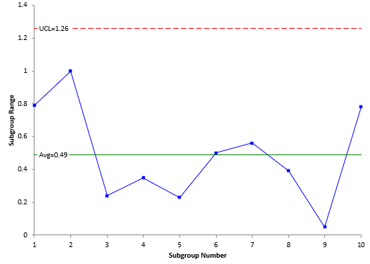
Each subgroup range is plotted in Figure 1. The subgroup range for subgroup 1 is the maximum result (11.46) minus the minimum result (10.67) or 11.46 – 10.67 = 0.79. What causes the variation in the results for subgroup 1? The same part is used for each of the three results. The variation in results is due to the measurement error or the test-retest error. The subgroup range calculations are repeated for each subgroup and each subgroup range is plotted on the chart.
Figure 1: Range Chart for Short EMP Study
In addition, the average subgroup range and the upper control limit are calculated. The next step is to interpret the range chart. Is it in statistical control? If there are no points beyond the control limits and no patterns, the range chart is in statistical control. The range chart in Figure1 is in statistical control. This means that the measurement variation is consistent from subgroup to subgroup.
If you have an out of control point, such as a point above the UCL, the range chart would not be in statistical control. In this case, the reason for the out of control point would have to be found and eliminated and the study repeated.
Since the measurement system is consistent, we can estimate the measurement error from the range chart. This is given by:
σe=R/d2
where σe is the measurement error, R is the average range, and d2 is a control chart constant that depends on subgroup size (n). As shown in Figure 1, the average range is 0.49. For a subgroup size of 3,d2= 1.693. Thus,
σe=R/d2= 0.49/1.693 = 0.29
Remember, if the range chart is not consistent, you can’t do this calculation.
X Control Chart Results
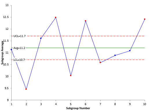
Each subgroup average is plotted in Figure 2. For example, the three results for subgroup 1 are averaged. The result is 11.13. This result represents the average for part 1. The same is done for the rest of the subgroups. So, the X chart is a plot of the part averages. The overall average is calculated as well as the upper control limit (UCL) and lower control limits (LCL).
Figure 2:X Chart for Short EMP Study
The control limit equations are:
UCL =X+ A2R
LCL =X– A2R
where X is the overall average and A2 is a control chart constant that depends on subgroup size. Note that R is used in the control limit equations. This average range represents the measurement error. The control limits on the X chart are based on the measurement system error. You hope that the measurement error is much less than the variation between the part averages. If this is true, then there should be out of control points on the X chart. Figure 2 does show out of control points.
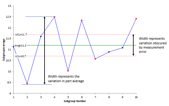
Since the X control limits are based on the measurement error, the width of the control limits represents the amount of part variation that is obscured by the measurement error. This is shown in Figure 3. You cannot see the variation in parts within these control limits because the variation is masked by the measurement error.
Figure 3: Measurement Error Impact on Part Average Variation
The figure also shows the width that is represented by the variation in the average of the parts. You want this width to be greater than the width obscured by the measurement error. This is true in Figure 3. You have indications from this chart that the measurement system can tell the difference between parts most of the time.
But, of course, we like to have statistics that describe how much – what percent of the total variation we see is due to the measurement system. This statistic can be calculated as shown below, and this opens other information you can get from a Short EMP Study.
Relationship between Total, Product and Measurement Variation
You sample your process on a regular basis. The samples are tested using your measurement process. You don’t get the same result each time you sample the process. Things vary. What are the sources of variation in the sample results? There are two major sources of variation: the variation in the product itself and the variation in the measurement system.
The basic equation describing the relationship between the total variance, the product variance and the measurement system variance is given below.
σx2=σp2+σe2
where σx2= total variance of the product measurements, σp2= the variance of the product, and σe2= the variance of the measurement system. There are two ratios that are used to help characterize the measurement process: the ratio of the product variance to the total variance and the ratio of the measurement system variance to the total variance.
Ratio of product variance to total variance = ρ =σp2/σx2
Ratio of measurement system variance to the total variance = 1 – ρ = σe2/σx2
ρ is the Intraclass Correlation Coefficient. Dr. Wheeler uses it to determine “how good” a measurement process is. To calculate these ratios, we need an estimate of the product variance. You can estimate the product variance for the EMP Short Study from the following equation:
σp2= sp2– σe2/n = 1.057 – (0.29)2/3 = 1.029
where sp2 is the pooled variance of the part averages. The table below shows the percentages for the two ratios:
Table 2: % of Variance Results for the Short EMP Study
| Source | Variance | % of Total |
|---|---|---|
| Measurement | 0.0841 | 7.56% |
| Product | 1.029 | 92.44% |
| Total | 1.1131 |
This shows that the % of total variance due to the measurement process Is 7.56% while the % of total variance due to the product variation 92.44%.
Other Insights for the EMP Short Study
Once you have the estimate of the measurement system error and these ratios, there are other things that can be determined.
- Classify the Measurement System
You can classify the measurement system (using the method developed by Dr. Wheeler) as a Class 1, Class 2, Class 3 or Class 4 monitor. This rating depends on the value of ρ, which is the % of variance due to the product. In this example, ρ = 92.44%. This classifies the measurement system as a Class 1 monitor. The classification system is based on the following criteria:
-
-
- How much the measurement system reduces a process signal
- The chance of detecting a ± 3 standard error shift
- The ability to track process improvements
-
This classification system is much better than the arbitrary methods used in the past that say the % Gage R&R must be less than some % of the total variation. This classification system is based on how the measurement system impacts the process. For more information on this classification system please see our SPC Knowledge Base article “Evaluating the Measurement Process – Part 1.”
- Determine the Number of Decimal Places to Record for the Measurement System
You can use the measurement system error (σe) to determine how many places you should record for the measurements. The probable error (PE) is used to do this:
PE = 0.675σe= 0.195
The measurement increment should be between 0.2(PE) and 2(PE), or between 0.039 and 0.39 for this example. The measurement increment in this example is 0.01, which is less than 0.039. This tells you that the measurement increment should be increased. For more information on this, please see our SPC Knowledge Base article “Probable Error and Your Measurement System.”
- Determine Internal Manufacturing Specifications
You can use the measurement error information to determine internal manufacturing specifications. For example, you can use the probable error to create 96% manufacturing specifications. The 96% is the probability that a part with a measured value between the manufacturing lower and upper specification limits conforms to specifications. You can also determine the Precision to Tolerance ratio which gives you the amount of specifications consumed by the measurement error. For more information on this, please see our SPC Knowledge Base article “Specifications and Measurement Error.”
Summary
This article introduced the Short EMP Study. This study involves an operator measuring multiple parts multiple times. The resulting analysis allows you to “see” how much of the variation in parts is obscured by the measurement error. The analysis estimates the measurement error as well as the product variance so that the % of variance due to the measurement system can be determined. This in turn opens other insights into the measurement system.
SPC for Excel Version 6 is Now Available


