March 2020
(Note: all the previous SPC Knowledge Base in the measurement systems analysis category are listed on the right-hand side. Select this link for information on the SPC for Excel software.)
This publication focuses on the first reason and how a statistic called the “precision to tolerance ratio” has been used to determine if a measurement system can detect if a part is within specifications. This publication examines two different approaches to determining the “precision to tolerance ratio.”
One approach, often attributed to AAIG (Automotive Action Industry Group), compares the measurement error spread to the tolerance. This is the most common approach and is responsible for untold amounts of money being spent to improve or purchase new measurement systems unnecessarily. This approach drastically overstates the impact of measurement error on the specifications.
The second approach, developed by Dr. Donald Wheeler, defines the precision-to-tolerance ratio as the amount of tolerance that is consumed by adjusting the specification limits to account for measurement error. This approach represents what happens in reality with measurement error’s impact on the specifications.
In this issue:
- Introduction
- Example Data
- AIAG Precision to Tolerance Ratio
- Dr. Wheeler’s Precision to Tolerance Ratio
- Summary
- Quick Links
You may download a pdf copy of this publication at this link. Please feel free to leave a comment at the end of the publication.
Introduction
One reason we take measurements is to see if our product is within specifications. Consider the following two scenarios:
- You take a sample from your process and measure it. The result is right below the upper specification limit (USL). What do you do? If you are like most of us, you assume it is within specifications. It is a good sample.
- You take a sample again from your process and measure it. The result is right above the USL. What do you do? Again, if you are like most of us, you either have the sample retested or you sample the process again. If the next result is within the USL, you assume it is good. If it is not, you assume it is out of specifications.
There is probably very little difference between the sample that was just above the USL and the one that was just below it. But our response is totally different because of the specification.
There is variation in our process, including the measurement system. Remeasuring the same part time and time again seldom gives the same result each time. Let’s look at some of the math we will need for this publication.
You take a sample from your process. You test that sample using your measurement system. You get a result (X1). You take another sample and test that sample. You get another result (X2). Usually X1 does not equal X2. What are the sources of variation in these results? Two major components of variation are present in each result: the variation in the product itself and the variation in the measurement system.
The basic equation describing the relationship between the total variance, the product variance and the measurement system variance is given below.
σx2= σp2+σe2
whereσx2= the total variance of the product measurements,σp2= the variance of the product, andσe2= the variance of the measurement system.
We will come back to this equation as we examine the two approaches for the precision to tolerance ratio (P/T).
Example Data
The P/T often comes up as part of a Gage R&R analysis. Suppose we perform a Gage R&R analysis on a measurement system used in our process. We select 3 operators (A, B, and C) to be part of the study. We select five parts that represent the spread of the production process. Each part is measured twice by each operator. The results are given in Table 1.
Table 1: Gage R&R Results
| Operator | Part | Result 1 | Result 2 |
|---|---|---|---|
| A | 1 | 257 | 252 |
| A | 2 | 300 | 303 |
| A | 3 | 277 | 273 |
| A | 4 | 279 | 286 |
| A | 5 | 246 | 237 |
| B | 1 | 245 | 247 |
| B | 2 | 296 | 289 |
| B | 3 | 272 | 269 |
| B | 4 | 274 | 268 |
| B | 5 | 233 | 232 |
| C | 1 | 242 | 245 |
| C | 2 | 296 | 293 |
| C | 3 | 270 | 271 |
| C | 4 | 270 | 272 |
| C | 5 | 236 | 244 |
These Gage R&R results can be analyzed using the Basic EMP Study method, the ANOVA method or the Average and Range method. All of these are covered in articles in our SPC Knowledge Base. To explore the AIAG P/T, we will need the results from the ANOVA or Average and Range method. To explore Dr. Wheeler’s P/T, we will need the results of the Basic EMP study. The ANOVA method and Basic EMP study were run using the SPC for Excel software. The detailed reports can be downloaded here for the ANOVA method and here for the Basic EMP study.
The numerical results for the variances in the equation above are very similar as shown in Table 2. The first column gives the source of the variation. The second and third columns are the results from the ANOVA Gage R&R method. The fourth and fifth columns are the results from the basic EMP study.
Table 2: ANOVA Gage R&R and Basic EMP Study Variances
| ANOVA Method | Basic EMP Study | |||
|---|---|---|---|---|
| Source | Variance | % Contribution | Variance | % of Total |
| Gage R&R | 31.97 | 5.68% | 33.65 | 5.96% |
| Repeatability | 12.45 | 2.21% | 14.31 | 2.54% |
| Reproducibility | 19.53 | 3.47% | 19.34 | 3.43% |
| Part-to-Part | 530.9 | 94.32% | 530.6 | 94.04% |
| Total Variance | 562.9 | 100.00% | 564.2 |
The measurement system error has two components: repeatability, which is the error due to the test itself, and reproducibility, which is the operator error . You combined these to get the total measurement error due to the repeatability of the test method and the differences in operators.
Now we are ready to explore the two P/T values. To do that, we need to know the process specifications. The LSL is 225 and the USL is 305.
AIAG Precision to Tolerance Ratio
The AIAG P/T is very simple. Mathematically, it is expressed as the following:
P/T=(6σe)/(USL-LSL)
where USL is the upper specification limit and LSL is the lower specification limit. The measurement standard deviation is multiplied by 6; this gives the “spread” of the measurement error. This “spread” is then divided by the tolerance, USL – LSL, to obtain the P/T value. The P/T value is often interpreted as the spread of the tolerance that is “consumed” by the measurement error.
AIAG provides the following guidelines for what acceptable and unacceptable P/T values are:
- Under 0.10: generally considered to be an acceptable measurement system
- 0.10 – 0.30: may be acceptable for some applications
- Over 0.30: considered to be unacceptable
These criteria are quite arbitrary – as evidence by the fact that the same criteria are used for the fraction of variation due to Gage R&R when using the standard deviations to do the calculations. For more information on this, please see our SPC Knowledge Base article Acceptance Criteria for Measurement Systems Analysis (MSA).
From the example data above, se is the square root of the variance due to Gage R&R (31.97) = 5.654, so the P/T value is:
In the ANOVA Gage R&R method report, this is referred to as the % of study variation/tolerance.
The way this is interpreted is usually that the measurement error consumes 42% of the tolerance. Under the AIAG guidelines, this is unacceptable. In fact, AIAG’s measurement systems analysis book says every effort should be made to improve the measurement system.
Let’s take a closer look at this approach to P/T. First, the value of 6 used to be 5.15. The value of 5.15 represented 99% of the standard normal distribution. The value of 6 represents 99.73%, or essentially all the data. Interesting when they changed from 5.15 to 6, they didn’t change the acceptance criteria above.
The equation for P/T above seems simple. But there is an issue with how we interpret it when we look a little closer. And we go back to the variance equation above to do that.
According to Dr. Wheeler, the “Intraclass Correlation Coefficient” is the traditional measure of association used to characterize the relative usefulness of a measurement system. The Intraclass Correlation Coefficient is simply the ratio of the product variance to the total variance and is denoted by ρ:
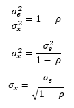
This is simply the % of the total variance that is due to the product variance. Remembering the basic variance equation above, then 1 –ρ is the % of the total variance that is due to the measurement system.
The product variance is not easy to estimate so the value of ρ is usually rewritten to be:
So, ρ is 1 minus the % of variance due to the measurement system.
It turns out that we can look at the influence of ρ on the process capability. The following math can be done:
Process capability is given by:
Substituting in σx gives the following:
Recognizing that the first part of the right-hand side of the equation is the inverse of P/T gives:
So, it turns out that P/T is related to the process capability index, Cp.
The value of P/T will remain constant for a set of specifications and a given measurement system. Now, suppose you improve the process, i.e., decrease the product variation. What happens to the above equation? Well, ρ decreases since it is the ratio of the product variance to the total variance. P/T is constant. So, Cp increases. This continues as more process improvements occur. As ρ approaches zero, the value of Cp will increase towards an upper bound that is defined by the inverse of P/T. But ρ cannot be zero, there is always variation.
So, the inverse of P/T is an upper bound on Cp that can’t be reached. Or vice-versa, P/T is the inverse of a number that can’t be reached. So, how can you explain what P/T means in terms of the process? You can’t. It has no meaning. All it means is that the measurement spread is some % of the tolerance. But it means nothing in terms of how the measurement error impacts if a part is within specifications, which is how we use specifications. More is needed.
Dr. Wheeler’s Precision to Tolerance Ratio
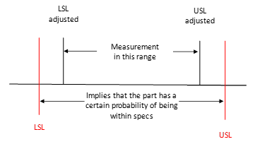
The approach below is described in detail in Dr. Wheeler’s book EMP III, Evaluating the Measurement Process and Using Imperfect Data. If this book is not on your bookshelf, it should be. Dr. Wheeler’s approach to P/T is to adjust the specifications to account for measurement error. The idea is shown in Figure 1.
Figure 1: Adjusting Specifications to Account for Measurement Error
The first question is how much to adjust the specifications. Dr. Wheeler uses the Probable Error (PE) to make the adjustments to the specifications. The Probable Error (PE) is defined as the following:
PE = 0.675σe
What is special about the value of PE? The PE defines the middle 50% of the normal distribution. This means that if you take repeated measurements on a sample, half of those repeated measurements should fall between the average and ± one PE. In this example, we will use the measurement system error from both the test and the operators (5.654)
Another thing that Dr. Wheeler introduces in this process the is concept of Watershed Specifications. Watershed Specifications are the specifications adjusted for the measurement increment. In the example above, the specifications are 225 to 305. The measurement increment is 1 as shown in Table 1. A test result of 225 is in spec, but a test result of 224 is not in spec. The Lower Watershed Specification Limit (LWSL) is defined as follows:
LWSL = LSL – Measurement Increment/2 = 225 – 1/2 = 224.5
The Upper Watershed Specification Limit (UWSL) is defined similarly:
UWSL = USL + Measurement Increment/2 = 305 + 1/2 = 305.5
So, the Watershed Specifications are essentially adjusting the customer specifications to account for the measurement increment. The Watershed Specification Limits are used to set the manufacturing specifications. For more information on this, please see our SPC Knowledge Base article on Specifications and Measurement Error.
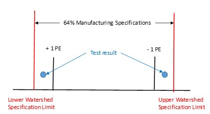
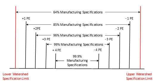
Suppose we decide to set our manufacturing specifications equal to the Watershed Specification Limits. Suppose a measurement is within the +/- 1 PE of the specification as shown in Figure 2.
Figure 2: 64% Manufacturing Specifications
Dr. Wheeler shows in his book that there is at least a 64% chance that the part is within specifications. Dr. Wheeler phrases it this way: “If you use your Watershed Specification Limits as your Manufacturing Specifications, you will have at least a 64 percent chance that the measured item is in spec when the measurement falls within the Manufacturing Specifications.”
This is not a very high percentage. You increase that by tightening the manufacturing specifications by moving them in by a given PE. Figure 3 shows how this works.
Figure 3: Manufacturing Specs and Probable Error
To see what this does for P/T, we will use the 96% manufacturing specifications. These are obtained by moving each of the Watershed Specifications in by 2 PE. So, the manufacturing specs are given by:
Lower Manufacturing Specification = 224.5 + 2PE = 224.5+2(0.675)(5.654) = 232.13
Upper Manufacturing Specification = 305.5 – 2PE = 305.5+2(0.675)(5.654) = 297.87
The question now becomes:
How much of the tolerance was consumed by moving to 96% manufacturing specifications?
This is a true measure of how much the measurement error impacts how we use the specifications. We have used up 4PE of the tolerance. So, the P/T value is given by:
Now compare this P/T value to the value obtained using AIAG’s approach: 42.4%. A much different number. The approach outlined using the Watershed Specifications represents what really happens in the world. It is a much more accurate picture of how the specification and measurement error interact. The AIAG P/T value overestimates the impact of measurement error on the specifications. It should not be used to judge “how good” a measurement system is.
Summary
This publication examined two methods for determining the P/T ratio: one from AIAG and one from Dr. Wheeler. AIAG’s method simply calculates a ratio of the measurement error spread to the tolerance and places artificial guidelines on what is acceptable and what is not. This method tends to overestimate the impact of measurement error on the specifications.
Dr. Wheeler’s approach uses the Watershed Specifications and the probable error to create manufacturing specifications that give you a probability of a part being in spec when the measurement lies between the upper and lower manufacturing specifications (e.g. 96%). The amount of tolerance that is consumed by moving the manufacturing specifications is then used to determine the P/T. This gives a much more accurate method of estimating the impact of measurement error on specifications.




Thank you very much for your calculation model. It makes clear how to prepare the internal release specifications.Congratulations, robust work.
very useful and relevant topic . thanks
Thank you very much for the explanations. But I have one question: when running the R&R study, sould I consider the product specification or the process specification? I mean, for example, if I have a product that its drawing/specification defines a thickness range of 0.008" – 0.014". But my inspection procedure defines a thighter range for security (process specification), let's say 0,009" – 0.013". What tolerance should I use to calculate my R&R results?
It depends on who the "customer" is for the Cpk analysis. Your external customer, you use the customer spec; for you, you use the internal specs.
Hello Dr. McNeese,
It seems that the AIAG MSA manual has many such misinterpreted ratios and yet when I google critiques of AIAG MSA methods, I don’t find very much out there. To me the math speaks for itself, however many of my colleagues are dubious or don’t have a background in math or stats and if they don’t downright insist on following the AIAG MSA manual, then they ask why has AIAG been accepted as a de facto “standard” in many industries. I don’t have a good reply for them nor a list of contradicting critiques. I know that when I was in the semiconductor industry, we followed SEMATECH and ISMI methods which were supported mathematically and were in direct conflict with some of the AIAG MSA methods. Do you know of such a list of critiques or how one may go about acquiring such a list?
Best regards,
Dan
Hello Dan,
We have a number of articles on our SPC Knowledge Base that discuss this. This one discussed the accepance criteria:
https://www.spcforexcel.com/knowledge/measurement-systems-analysis/acceptance-criteria-for-msa/
Dr. Wheeler is one who has really critized AIAG’s approach. Here is a good article from him:
https://www.spcpress.com/pdf/DJW189.pdf
Best Regards,
Bill